


In this chapter, we examine the representation of dynamic sets by simple data structures that use pointers. Although many complex data structures can be fashioned using pointers, we present only the rudimentary ones: stacks, queues, linked lists, and rooted trees. We also discuss a method by which objects and pointers can be synthesized from arrays.
Stacks and queues are dynamic sets in which the element removed from the set by the DELETE operation is prespecified. In a stack, the element deleted from the set is the one most recently inserted: the stack implements a last-in, first-out, or LIFO, policy. Similarly, in a queue , the element deleted is always the one that has been in the set for the longest time: the queue implements a first-in, first-out, or FIFO, policy. There are several efficient ways to implement stacks and queues on a computer. In this section we show how to use a simple array to implement each.
The INSERT operation on a stack is often called PUSH, and the DELETE operation, which does not take an element argument, is often called POP. These names are allusions to physical stacks, such as the spring-loaded stacks of plates used in cafeterias. The order in which plates are popped from the stack is the reverse of the order in which they were pushed onto the stack, since only the top plate is accessible.
As shown in Figure 11.1, we can implement a stack of at most n elements with an array S [1..n]. The array has an attribute top[S] that indexes the most recently inserted element. The stack consists of elements S[1..top[S]], where S[1] is the element at the bottom of the stack and S[top[S]] is the element at the top.
When top [S] = 0, the stack contains no elements and is empty. The stack can be tested for emptiness by the query operation STACK-EMPTY. If an empty stack is popped, we say the stack underflows, which is normally an error. If top[S] exceeds n, the stack overflows. (In our pseudocode implementation, we don't worry about stack overflow.)
The stack operations can each be implemented with a few lines of code.
Figure 11.1 shows the effects of the modifying operations PUSH and POP. Each of the three stack operations takes O (1) time.
We call the INSERT operation on a queue ENQUEUE, and we call the DELETE operation DEQUEUE; like the stack operation POP, DEQUEUE takes no element argument. The FIFO property of a queue causes it to operate like a line of people in the registrar's office. The queue has a head and a tail. When an element is enqueued, it takes its place at the tail of the queue, 1ike a newly arriving student takes a place at the end of the line. The element dequeued is always the one at the head of the queue, like the student at the head of the line who has waited the longest. (Fortunately, we don't have to worry about computational elements cutting into line.)
Figure 11.2 shows one way to implement a queue of at most n - 1 elements using an array Q [1..n]. The queue has an attribute head [Q] that indexes, or points to, its head. The attribute tail [Q] indexes the next location at which a newly arriving element will be inserted into the queue. The elements in the queue are in locations head[Q], head [Q] + 1, . . . , tail [Q] - 1, where we "wrap around" in the sense that location 1 immediately follows location n in a circular order. When head [Q] = tail [Q], the queue is empty. Initially, we have head [Q] = tail [Q] = 1. When the queue is empty, an attempt to dequeue an element causes the queue to underflow. When head [Q] = tail [Q] + 1, the queue is full, and an attempt to enqueue an element causes the queue to overflow.
In our procedures ENQUEUE and DEQUEUE, the error checking for underflow and overflow has been omitted. (Exercise 11.1-4 asks you to supply code that checks for these two error conditions.)
Figure 11.2 shows the effects of the ENQUEUE and DEQUEUE operations. Each operation takes O(1) time.
11.1-1
Using Figure 11.1 as a model, illustrate the result of each of the operations PUSH(S, 4), PUSH(S, 1), PUSH(S, 3), POP(S), PUSH(S, 8), and POP(S) on an initially empty stack S stored in array S [1 . . 6].
11.1-2
Explain how to implement two stacks in one array A [1 . . n] in such a way that neither stack overflows unless the total number of elements in both stacks together is n. The PUSH and POP operations should run in O(1) time.
11.1-3
Using Figure 11.2 as a model, illustrate the result of each of the operations ENQUEUE(Q, 4), ENQUEUE(Q, 1), ENQUEUE(Q, 3), DEQUEUE(Q), ENQUEUE(Q, 8), and DEQUEUE(Q) on an initially empty queue Q stored in array Q [1 . . 6].
11.1-4
Rewrite ENQUEUE and DEQUEUE to detect underflow and overflow of a queue.
11.1-5
Whereas a stack allows insertion and deletion of elements at only one end, and a queue allows insertion at one end and deletion at the other end, a deque (double-ended queue) allows insertion and deletion at both ends. Write four O(1)-time procedures to insert elements into and delete elements from both ends of a deque constructed from an array.
11.1-6
Show how to implement a queue using two stacks. Analyze the running time of the queue operations.
11.1-7
Show how to implement a stack using two queues. Analyze the running time of the stack operations.
A linked list is a data structure in which the objects are arranged in a linear order. Unlike an array, though, in which the linear order is determined by the array indices, the order in a linked list is determined by a pointer in each object. Linked lists provide a simple, flexible representation for dynamic sets, supporting (though not necessarily efficiently) all the operations listed on page 198.
As shown in Figure 11.3, each element of a doubly linked list L is an object with a key field and two other pointer fields: next and prev. The object may also contain other satellite data. Given an element x in the list, next [x] points to its successor in the linked list, and prev [x] points to its predecessor. If prev [x] = NIL, the element x has no predecessor and is therefore the first element, or head, of the list. If next [x] = NIL, the element x has no successor and is therefore the last element, or tail, of the list. An attribute head [L] points to the first element of the list. If head [L] = NIL, the list is empty.
A list may have one of several forms. It may be either singly linked or doubly linked, it may be sorted or not, and it may be circular or not. If a list is singly linked, we omit the prev pointer in each element. If a list is sorted, the linear order of the list corresponds to the linear order of keys stored in elements of the list; the minimum element is the head of the list, and the maximum element is the tail. If the list is unsorted, the elements can appear in any order. In a circular list, the prev pointer of the head of the list points to the tail, and the next pointer of the tail of the list points to the head. The list may thus be viewed as a ring of elements. In the remainder of this section, we assume that the lists with which we are working are unsorted and doubly linked.
The procedure LIST-SEARCH(L, k) finds the first element with key k in list L by a simple linear search, returning a pointer to this element. If no object with key k appears in the list, then NIL is returned. For the linked list in Figure 11.3(a), the call LIST-SEARCH(L, 4) returns a pointer to the third element, and the call LIST-SEARCH(L, 7) returns NIL.
To search a list of n objects, the LIST-SEARCH procedure takes
Given an element x whose key field has already been set, the LIST-INSERT procedure "splices" x onto the front of the linked list, as shown in Figure 11.3(b).
The running time for LIST-INSERT on a list of n elements is O(1).
The procedure LIST-DELETE removes an element x from a linked list L. It must be given a pointer to x, and it then "splices" x out of the list by updating pointers. If we wish to delete an element with a given key, we must first call LIST-SEARCH to retrieve a pointer to the element.
Figure 11.3(c) shows how an element is deleted from a linked list. LIST-DELETE runs in O(1) time, but if we wish to delete an element with a given key,
The code for LIST-DELETE would be simpler if we could ignore the boundary conditions at the head and tail of the list.
A sentinel is a dummy object that allows us to simplify boundary conditions. For example, suppose that we provide with list L an object nil[L] that represents NIL but has all the fields of the other list elements. Wherever we have a reference to NIL in list code, we replace it by a reference to the sentinel nil[L]. As shown in Figure 11.4, this turns a regular doubly linked list into a circular list, with the sentinel nil[L] placed between the head and tail; the field next[nil[L]] points to the head of the list, and prev[nil[L]] points to the tail. Similarly, both the next field of the tail and the prev field of the head point to nil[L]. Since next[nil[L]] points to the head, we can eliminate the attribute head[L] altogether, replacing references to it by references to next[nil[L]]. An empty list consists of just the sentinel, since both next[nil[L]] and prev[nil[L]] can be set to nil[L].
The code for LIST-SEARCH remains the same as before, but with the references to NIL and head[L] changed as specified above.
We use the two-line procedure LIST-DELETE' to delete an element from the list. We use the following procedure to insert an element into the list.
Figure 11.4 shows the effects of LIST-INSERT' and LIST-DELETE' on a sample list.
Sentinels rarely reduce the asymptotic time bounds of data structure operations, but they can reduce constant factors. The gain from using sentinels within loops is usually a matter of clarity of code rather than speed; the linked list code, for example, is simplified by the use of sentinels, but we save only O(1) time in the LIST-INSERT' and LIST-DELETE' procedures. In other situations, however, the use of sentinels helps to tighten the code in a loop, thus reducing the coefficient of, say, n or n2 in the running time.
Sentinels should not be used indiscriminately. If there are many small lists, the extra storage used by their sentinels can represent significant wasted memory. In this book, we only use sentinels when they truly simplify the code.
11.2-1
Can the dynamic-set operation INSERT be implemented on a singly linked list in O(1) time? How about DELETE?
11.2-2
Implement a stack using a singly linked list L. The operations PUSH and POP should still take O(1) time.
11.2-3
Implement a queue by a singly linked list L. The operations ENQUEUE and DEQUEUE should still take O(1) time.
11.2-4
Implement the dictionary operations INSERT, DELETE, and SEARCH using singly linked, circular lists. What are the running times of your procedures?
11.2-5
The dynamic-set operation UNION takes two disjoint sets Sl and S2 as input, and it returns a set S = S1
11.2-6
Write a procedure that merges two singly linked, sorted lists into one singly linked, sorted list without using sentinels. Then, write a similar procedure using a sentinel with key
11.2-7
Give a
11.2-8
Explain how to implement doubly linked lists using only one pointer value np[x] per item instead of the usual two (next and prev). Assume that all index values can be interpreted as k-bit integers, and define np[x] to be np[x] = next[x] XOR prev[x], the k-bit "exclusive-or" of next[x] and prev[x]. (The value NIL is represented by 0.) Be sure to describe what information is needed to access the head of the list. Show how to implement the SEARCH, INSERT, and DELETE operations on such a list. Also show how to reverse such a list in O(1) time.
How do we implement pointers and objects in languages, such as Fortran, that do not provide them? In this section, we shall see two ways of implementing linked data structures without an explicit pointer data type. We shall synthesize objects and pointers from arrays and array indices.
We can represent a collection of objects that have the same fields by using an array for each field. As an example, Figure 11.5 shows how we can implement the linked list of Figure 11.3(a) with three arrays. The array key holds the values of the keys currently in the dynamic set, and the pointers are stored in the arrays next and prev. For a given array index x, key[x], next[x], and prev[x] represent an object in the linked list. Under this interpretation, a pointer x is simply a common index into the key, next, and prev arrays.
In Figure 11.3(a), the object with key 4 follows the object with key 16 in the linked list. In Figure 11.5, key 4 appears in key[2], and key 16 appears in key[5], so we have next[5] = 2 and prev[2] = 5. Although the constant NIL appears in the next field of the tail and the prev field of the head, we usually use an integer (such as 0 or -1) that cannot possibly represent an actual index into the arrays. A variable L holds the index of the head of the list.
In our pseudocode, we have been using square brackets to denote both the indexing of an array and the selection of a field (attribute) of an object. Either way, the meanings of key[x], next[x], and prev[x] are consistent with implementation practice.
The words in a computer memory are typically addressed by integers from 0 to M - 1, where M is a suitably large integer. In many programming languages, an object occupies a contiguous set of locations in the computer memory. A pointer is simply the address of the first memory location of the object, and other memory locations within the object can be indexed by adding an offset to the pointer.
We can use the same strategy for implementing objects in programming environments that do not provide explicit pointer data types. For example, Figure 11.6 shows how a single array A can be used to store the linked list from Figures 11.3(a) and 11.5. An object occupies a contiguous subarray A[j . . k]. Each field of the object corresponds to an offset in the range from 0 to k - j, and a pointer to the object is the index j. In Figure 11.6, the offsets corresponding to key, next, and prev are 0, 1, and 2, respectively. To read the value of prev[i], given a pointer i, we add the value i of the pointer to the offset 2, thus reading A[i + 2].
The single-array representation is flexible in that it permits objects of different lengths to be stored in the same array. The problem of managing such a heterogeneous collection of objects is more difficult than the problem of managing a homogeneous collection, where all objects have the same fields. Since most of the data structures we shall consider are composed of homogeneous elements, it will be sufficient for our purposes to use the multiple-array representation of objects.
To insert a key into a dynamic set represented by a doubly linked list, we must allocate a pointer to a currently unused object in the linked-list representation. Thus, it is useful to manage the storage of objects not currently used in the linked-list representation so that one can be allocated. In some systems, a garbage collector is responsible for determining which objects are unused. Many applications, however, are simple enough that they can bear responsibility for returning an unused object to a storage manager. We shall now explore the problem of allocating and freeing (or deallocating) homogeneous objects using the example of a doubly linked list represented by multiple arrays.
Suppose that the arrays in the multiple-array representation have length m and that at some moment the dynamic set contains n
We keep the free objects in a singly linked list, which we call the free list. The free list uses only the next array, which stores the next pointers within the list. The head of the free list is held in the global variable free. When the dynamic set represented by linked list L is nonempty, the free list may be intertwined with list L, as shown in Figure 11.7. Note that each object in the representation is either in list L or in the free list, but not in both.
The free list is a stack: the next object allocated is the last one freed. We can use a list implementation of the stack operations PUSH and POP to implement the procedures for allocating and freeing objects, respectively.
We assume that the global variable free used in the following procedures points to the first element of the free list.
The free list initially contains all n unallocated objects. When the free list has been exhausted, the ALLOCATE-OBJECT procedure signals an error. It is common to use a single free list to service several linked lists. Figure 11.8 shows three linked lists and a free list intertwined through key, next, and prev arrays.
The two procedures run in O(1) time, which makes them quite practical. They can be modified to work for any homogeneous collection of objects by letting any one of the fields in the object act like a next field in the free list.
11.3-1
Draw a picture of the sequence
11.3-2
Write the procedures ALLOCATE-OBJECT and FREE-OBJECT for a homogeneous collection of objects implemented by the single-array representation.
11.3-3
Why don't we need to set or reset the prev fields of objects in the implementation of the ALLOCATE-OBJECT and FREE-OBJECT procedures?
11.3-4
It is often desirable to keep all elements of a doubly linked list compact in storage, using, for example, the first m index locations in the multiple-array representation. (This is the case in a paged, virtual-memory computing environment.) Explain how the procedures ALLOCATE-OBJECT and FREE-OBJECT can be implemented so that the representation is compact. Assume that there are no pointers to elements of the linked list outside the list itself. (Hint: Use the array implementation of a stack.)
11.3-5
Let L be a doubly linked list of length m stored in arrays key, prev, and next of length n. Suppose that these arrays are managed by ALLOCATE-OBJECT and FREE-OBJECT procedures that keep a doubly linked free list F. Suppose further that of the n items, exactly m are on list L and n - m are on the free list. Write a procedure COMPACTIFY-LIST (L, F) that, given the list L and the free list F, moves the items in L so that they occupy array positions 1, 2, . . . , m and adjusts the free list F so that it remains correct, occupying array positions m + 1, m + 2, . . . , n. The running time of your procedure should be
The methods for representing lists given in the previous section extend to any homogeneous data structure. In this section, we look specifically at the problem of representing rooted trees by linked data structures. We first look at binary trees, and then we present a method for rooted trees in which nodes can have an arbitrary number of children.
We represent each node of a tree by an object. As with linked lists, we assume that each node contains a key field. The remaining fields of interest are pointers to other nodes, and they vary according to the type of tree.
As shown in Figure 11.9, we use the fields p, left, and right to store pointers to the parent, left child, and right child of each node in a binary tree T. If p[x] = NIL, then x is the root. If node x has no left child, then left[x] = NIL, and similarly for the right child. The root of the entire tree T is pointed to by the attribute root[T]. If root [T] = NIL, then the tree is empty.
The scheme for representing a binary tree can be extended to any class of trees in which the number of children of each node is at most some constant k: we replace the left and right fields by child1, child2, . . . , childk. This scheme no longer works when the number of children of a node is unbounded, since we do not know how many fields (arrays in the multiple-array representation) to allocate in advance. Moreover, even if the number of children k is bounded by a large constant but most nodes have a small number of children, we may waste a lot of memory.
Fortunately, there is a clever scheme for using binary trees to represent trees with arbitrary numbers of children. It has the advantage of using only O(n) space for any n-node rooted tree. The left-child, right-sibling representation is shown in Figure 11.10. As before, each node contains a parent pointer p, and root[T] points to the root of tree T. Instead of having a pointer to each of its children, however, each node x has only two pointers:
1. left-child[x] points to the leftmost child of node x, and
2. right-sibling[x] points to the sibling of x immediately to the right.
If node x has no children, then left-child[x] = NIL, and if node x is the rightmost child of its parent, then right-sibling[x] = NIL.
We sometimes represent rooted trees in other ways. In Chapter 7, for example, we represented a heap, which is based on a complete binary tree, by a single array plus an index. The trees that appear in Chapter 22 are only traversed toward the root, so only the parent pointers are present; there are no pointers to children. Many other schemes are possible. Which scheme is best depends on the application.
11.4-1
Draw the binary tree rooted at index 6 that is represented by the following fields.
11.4-2
Write an O(n)-time recursive procedure that, given an n-node binary tree, prints out the key of each node in the tree.
11.4-3
Write an O(n)-time nonrecursive procedure that, given an n-node binary tree, prints out the key of each node in the tree. Use a stack as an auxiliary data structure.
11.4-4
Write an O(n)-time procedure that prints all the keys of an arbitrary rooted tree with n nodes, where the tree is stored using the left-child, right-sibling representation.
11.4-5
Write an O(n)-time nonrecursive procedure that, given an n-node binary tree, prints out the key of each node. Use no more than constant extra space outside of the tree itself and do not modify the tree, even temporarily, during the procedure.
11.4-6
The left-child, right-sibling representation of an arbitrary rooted tree uses three pointers in each node: left-child, right-sibling, and parent. From any node, the parent and all the children of the node can be reached and identified. Show how to achieve the same effect using only two pointers and one boolean value in each node.
11-1 Comparisons among lists
For each of the four types of lists in the following table, what is the asymptotic worst-case running time for each dynamic-set operation listed?
11-2 Mergeable heaps using linked lists
A mergeable heap supports the following operations: MAKE-HEAP (which creates an empty mergeable heap), INSERT, MINIMUM, EXTRACT-MIN, and UNION. Show how to implement mergeable heaps using linked lists in each of the following cases. Try to make each operation as efficient as possible. Analyze the running time of each operation in terms of the size of the dynamic set(s) being operated on.
a. Lists are sorted.
b. Lists are unsorted.
c. Lists are unsorted, and dynamic sets to be merged are disjoint.
11-3 Searching a sorted compact list
Exercise 11.3-4 asked how we might maintain an n-element list compactly in the first n positions of an array. We shall assume that all keys are distinct and that the compact list is also sorted, that is, key[i] < key[next[i]] for all i = 1, 2, . . . , n such that next[i]
If we ignore lines 4-6 of the procedure, we have the usual algorithm for searching a sorted linked list, in which index i points to each position of the list in turn. Lines 4-6 attempt to skip ahead to a randomly chosen position j. Such a skip is beneficial if key[j] is larger than key[i] and smaller than k; in such a case, j marks a position in the list that i would have to pass by during an ordinary list search. Because the list is compact, we know that any choice of j between 1 and n indexes some object in the list rather than a slot on the free list.
a. Why do we assume that all keys are distinct in COMPACT-LIST-SEARCH? Argue that random skips do not necessarily help asymptotically when the list contains repeated key values.
We can analyze the performance of COMPACT-LIST-SEARCH by breaking its execution into two phases. During the first phase, we discount any progress toward finding k that is accomplished by lines 7-9. That is, phase 1 consists of moving ahead in the list by random skips only. Likewise, phase 2 discounts progress accomplished by lines 4-6, and thus it operates like ordinary linear search.
Let Xt be the random variable that describes the distance in the linked list (that is, through the chain of next pointers) from position i to the desired key k after t iterations of phase l.
b. Argue that the expected running time of COMPACT-LIST-SEARCH is O(t+E [Xt]) for all t
c. Show that
d. Show that
e. Prove that E[Xt]
f. Show that COMPACT-LIST-SEARCH runs in
Aho, Hopcroft, and Ullman [5] and Knuth [121] are excellent references for elementary data structures. Gonnet [90] provides experimental data on the performance of many data structure operations.
The origin of stacks and queues as data structures in computer science is unclear, since corresponding notions already existed in mathematics and paper-based business practices before the introduction of digital computers. Knuth [121] cites A. M. Turing for the development of stacks for subroutine linkage in 1947.
Pointer-based data structures also seem to be a folk invention. According to Knuth, pointers were apparently used in early computers with drum memories. The A-l language developed by G. M. Hopper in 1951 represented algebraic formulas as binary trees. Knuth credits the IPL-II language, developed in 1956 by A. Newell, J. C. Shaw, and H. A. Simon, for recognizing the importance and promoting the use of pointers. Their IPL-III language, developed in 1957, included explicit stack operations.
11.1 Stacks and queues
Stacks
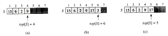
Figure 11.1 An array implementation of a stack S. Stack elements appear only in the lightly shaded positions. (a) Stack S has 4 elements. The top element is 9. (b) Stack S after the calls PUSH(S, 17) and PUSH(S, 3). (c) Stack S after the call POP(S) has returned the element 3, which is the one most recently pushed. Although element 3 still appears in the array, it is no longer in the stack; the top is element 17.
STACK-EMPTY(S)
1 if top [S] = 0
2 then return TRUE
3 else return FALSE
PUSH(S, x)
1 top[S]
 top [S] + 1
2 S [top[S]]
xPOP(S)
1 if STACK-EMPTY(S)
2 then error "underflow"
3 else top [S]
top [S] - 14 return S [top [S] + 1]
Queues
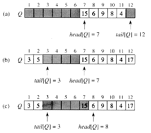
Figure 11.2 A queue implemented using an array Q[1 . . 12]. Queue elements appear only in the lightly shaded positions. (a) The queue has 5 elements, in locations Q [7..11]. (b) The configuration of the queue after the calls ENQUEUE(Q, 17), ENQUEUE(Q, 3), and ENQUEUE(Q, 5). (c) The configuration of the queue after the call DEQUEUE(Q) returns the key value 15 formerly at the head of the queue. The new head has key 6.
ENQUEUE(Q, x)
1 Q [tail [Q]]
x2 if tail [Q] = length [Q]
3 then tail [Q]
14 else tail [Q]
tail [Q] + 1DEQUEUE(Q)
1 x
Q [head [Q]]2 if head [Q] = length [Q]
3 then head [Q]
14 else head [Q]
head [Q] + 15 return x
Exercises
11.2 Linked lists
Searching a linked list
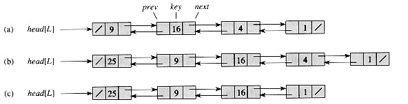
Figure 11.3 (a) A doubly linked list L representing the dynamic set {1, 4, 9, 16}. Each element in the list is an object with fields for the key and pointers (shown by arrows) to the next and previous objects. The next field of the tail and the prev field of the head are NIL, indicated by a diagonal slash. The attribute head[L] points to the head. (b) Following the execution of LIST-INSERT(L, x), where key[x] = 25, the linked list has a new object with key 25 as the new head. This new object points to the old head with key 9. (c) The result of the subsequent call LIST-DELETE(L, x), where x points to the object with key 4.
LIST-SEARCH(L, k)
1 x
head[L]2 while x
 NIL and key[x] k
3 do x
next[x]4 return x
 (n) time in the worst case, since it may have to search the entire list.
Inserting into a linked list
LIST-INSERT(L, x)
1 next[x]
head[L]2 if head[L]
NIL3 then prev[head[L]]
x4 head[L]
x5 prev[x]
NILDeleting from a linked list
LIST-DELETE(L, x)
1 if prev[x]
NIL2 then next[prev[x]]
next[x]3 else head[L]
next[x]4 if next[x]
NIL5 then prev[next[x]]
prev[x](n) time is required in the worst case because we must first call LIST-SEARCH.Sentinels
LIST-DELETE'(L, x)
1 next[prev[x]]
next[x]2 prev[next[x]]
prev[x]
Figure 11.4 A linked list L that uses a sentinel nil[L] (heavily shaded) is the regular doubly linked list turned into a circular list with nil[L] appearing between the head and tail. The attribute head[L] is no longer needed, since we can access the head of the list by next[nil[L]]. (a) An empty list. (b) The linked list from Figure 11.3(a), with key 9 at the head and key 1 at the tail. (c) The list after executing LIST-INSERT(L, x), where, key[x] = 25. The new object becomes the head of the list. (d) The list after deleting the object with key 1. The new tail is the object with key 4.
LIST-SEARCH'(L, k)
1 x
next[nil[L]]2 while x
nil[L] and key[x] k3 do x
next[x]4 return x
LIST-INSERT'(L, x)
1 next[x]
next[nil[L]]2 prev[next[nil[L]]]
x3 next[nil[L]]
x4 prev[x]
nil[L]Exercises
 S2 consisting of all the elements of S1 and S2. The sets S1 and S2 are usually destroyed by the operation. Show how to support UNION in O(1) time using a suitable list data structure.
 to mark the end of each list. Compare the simplicity of code for the two procedures.(n)-time nonrecursive procedure that reverses a singly linked list of n elements. The procedure should use no more than constant storage beyond that needed for the list itself.
11.3 Implementing pointers and objects
A multiple-array representation of objects

Figure 11.5 The linked list of Figure 11.3(a) represented by the arrays key, next, and prev. Each vertical slice of the arrays represents a single object. Stored pointers correspond to the array indices shown at the top; the arrows show how to interpret them. Lightly shaded object positions contain list elements. The variable L keeps the index of the head.

Figure 11.6 The linked list of Figures 11.3(a) and 11.5 represented in a single array A. Each list element is an object that occupies a contiguous subarray of length 3 within the array. The three fields key, next, and prev correspond to the offsets 0, 1, and 2, respectively. A pointer to an object is an index of the first element of the object. Objects containing list elements are lightly shaded, and arrows show the list ordering.
A single-array representation of objects
Allocating and freeing objects
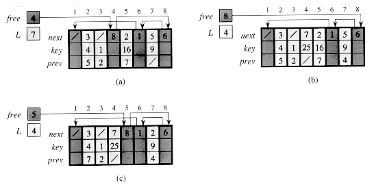
Figure 11.7 The effect of the ALLOCATE-OBJECT and FREE-OBJECT procedures. (a) The list of Figure 11.5 (lightly shaded) and a free list (heavily shaded). Arrows show the free-list structure. (b) The result of calling ALLOCATE-OBJECT() (which returns index 4), setting key[4] to 25, and calling LIST-INSERT(L, 4). The new free-list head is object 8, which had been next[4] on the free list. (c) After executing LIST-DELETE(L, 5), we call FREE-OBJECT(5). Object 5 becomes the new free-list head, with object 8 following it on the free list.
 m elements. Then n objects represent elements currently in the dynamic set, and the remaining m - n objects are free; the free objects can be used to represent elements inserted into the dynamic set in the future.
Figure 11.8 Two linked lists, L1 (lightly shaded) and L2 (heavily shaded), and a free list (darkened) intertwined.
ALLOCATE-OBJECT( )
1 if free = NIL
2 then error "out of space"
3 else x
free4 free
next[x]5 return x
FREE-OBJECT(x)
1 next[x]
free2 free
xExercises
 13, 4, 8, 19, 5, 11
 stored as a doubly linked list using the multiple-array representation. Do the same for the single-array representation.(m), and it should use only a constant amount of extra space. Give a careful argument for the correctness of your procedure.
11.4 Representing rooted trees
Binary trees

Figure 11.9 The representation of a binary tree T. Each node x has the fields p[x] (top), left[x] (lower left), and right[x] (lower right). The key fields are not shown.
Rooted trees with unbounded branching
Other tree representations

Figure 11.10 The left-child, right-sibling representation of a tree T. Each node x has fields p[x] (top), left-child[x] (lower left), and right-sibling[x] (lower right). Keys are not shown.
Exercises
index key left right
----------------------
1 12 7 3
2 15 8 NIL
3 4 10 NIL
4 10 5 9
5 2 NIL NIL
6 18 1 4
7 7 NIL NIL
8 14 6 2
9 21 NIL NIL
10 5 NIL NIL
Problems
unsorted, sorted, unsorted, sorted,
singly singly doubly doubly
linked linked linked linked
---------------------------------------------------------
SEARCH(L,k)
INSERT(L,x)
DELETE(L,x)
SUCCESSOR(L,x)
PREDECESSOR(L,x)
MINIMUM(L)
MAXIMUM(L)
NIL. Under these assumptions, we expect that the following randomized algorithm can be used to search the list much faster than linear time.COMPACT-LIST-SEARCH(L, k)
1 i
head[L]2 n
length[L]3 while i
NIL and key[i] < k4 do j
RANDOM(l, n)5 if key[i] < key[j] and key[j] < k
6 then i
j7 i
next[i]8 if key[i] = k
9 then return i
10 return NIL
 0.
0. . (Hint. Use equation (6.28).)
 n/(t + 1), and explain why this formula makes intuitive sense.
 expected time.
Chapter notes