


As parallel-processing computers have proliferated, interest has increased in parallel algorithms: algorithms that perform more than one operation at a time. The study of parallel algorithms has now developed into a research area in its own right. Indeed, parallel algorithms have been developed for many of the problems we have solved in this text using ordinary serial algorithms. In this chapter, we shall describe a few simple parallel algorithms that illustrate fundamental issues and techniques.
In order to study parallel algorithms, we must choose an appropriate model for parallel computing. The random-access machine, or RAM, which we have used throughout most of this book, is, of course, serial rather than parallel. The parallel models we have studied--sorting networks (Chapter 28) and circuits (Chapter 29)--are too restrictive for investigating, for example, algorithms on data structures.
The parallel algorithms in this chapter are presented in terms of one popular theoretical model: the parallel random-access machine, or PRAM (pronounced "PEE-ram"). Many parallel algorithms for arrays, lists, trees, and graphs can be easily described in the PRAM model. Although the PRAM ignores many important aspects of real parallel machines, the essential attributes of parallel algorithms tend to transcend the models for which they are designed. If one PRAM algorithm outperforms another PRAM algorithm, the relative performance is not likely to change substantially when both algorithms are adapted to run on a real parallel computer.
The PRAM model
Figure 30.1 shows the basic architecture of the parallel random-access machine (PRAM). There are p ordinary (serial) processors P0, P1, . . . , Pp-1 that have as storage a shared, global memory. All processors can read from or write to the global memory "in parallel" (at the same time). The processors can also perform various arithmetic and logical operations in parallel.
The key assumption regarding algorithmic performance in the PRAM model is that running time can be measured as the number of parallel memory accesses an algorithm performs. This assumption is a straight- forward generalization of the ordinary RAM model, in which the number of memory accesses is asymptotically as good as any other measure of running time. This simple assumption will serve us well in our survey of parallel algorithms, even though real parallel computers cannot perform parallel accesses to global memory in unit time: the time for a memory access grows with the number of processors in the parallel computer.
Nevertheless, for parallel algorithms that access data in an arbitrary fashion, the assumption of unit-time memory operations can be justified. Real parallel machines typically have a communication network that can support the abstraction of a global memory. Accessing data through the network is a relatively slow operation in comparison with arithmetic and other operations. Thus, counting the number of parallel memory accesses executed by two parallel algorithms does, in fact, yield a fairly accurate estimate of their relative performances. The principal way in which real machines violate the unit-time abstraction of the PRAM is that some memory-access patterns are faster than others. As a first approximation, however, the unit-time assumption in the PRAM model is quite reasonable.
The running time of a parallel algorithm depends on the number of processors executing the algorithm as well as the size of the problem input. Generally, therefore, we must discuss both time and processor count when analyzing PRAM algorithms; this contrasts with serial algorithms, in whose analysis we have focused mainly on time. Typically, there is a trade-off between the number of processors used by an algorithm and its running time. Section 30.3 discusses these trade-offs.
Concurrent versus exclusive memory accesses
A concurrent-read algorithm is a PRAM algorithm during whose execution multiple processors can read from the same location of shared memory at the same time. An exclusive-read algorithm is a PRAM algorithm in which no two processors ever read the same memory location at the same time. We make a similar distinction with respect to whether or not multiple processors can write into the same memory location at the same time, dividing PRAM algorithms into concurrent-write and exclusive-write algorithms. Commonly used abbreviations for the types of algorithms we encounter are
(These abbreviations are usually pronounced not as words but rather as strings of letters.)
Of these types of algorithms, the extremes--EREW and CRCW--are the most popular. A PRAM that supports only EREW algorithms is called an EREW PRAM, and one that supports CRCW algorithms is called a CRCW PRAM. A CRCW PRAM can, of course, execute EREW algorithms, but an EREW PRAM cannot directly support the concurrent memory accesses required in CRCW algorithms. The underlying hardware of an EREW PRAM is relatively simple, and therefore fast, because it needn't handle conflicting memory reads and writes. A CRCW PRAM requires more hardware support if the unit-time assumption is to provide a reasonably accurate measure of algorithmic performance, but it provides a programming model that is arguably more straightforward than that of an EREW PRAM.
Of the remaining two algorithmic types--CREW and ERCW--more attention has been paid in the literature to the CREW. From a practical point of view, however, supporting concurrency for writes is no harder than supporting concurrency for reads. In this chapter, we shall generally treat an algorithm as being CRCW if it contains either concurrent reads or concurrent writes, without making further distinctions. We discuss the finer points of this distinction in Section 30.2.
When multiple processors write to the same location in a CRCW algorithm, the effect of the parallel write is not well defined without additional elaboration. In this chapter, we shall use the common-CRCW model: when several processors write into the same memory location, they must all write a common (the same) value. There are several alternative types of PRAM's in the literature that handle this problem with a different assumption. Other choices include
In the last case, the specified combination is typically some associative and commutative function such as addition (store the sum of all the values written) or maximum (store only the maximum value written).
Synchronization and control
PRAM algorithms must be highly synchronized to work correctly. How is this synchronization achieved? Also, the processors in PRAM algorithms must often detect termination of loop conditions that depend on the state of all processors. How is this control function implemented?
We won't discuss these issues extensively. Many real parallel computers employ a control network connecting the processors that helps with synchronization and termination conditions. Typically, the control network can implement these functions as fast as a routing network can implement global memory references.
For our purposes, it suffices to assume that the processors are inherently tightly synchronized. All processors execute the same statements at the same time. No processor races ahead while others are further back in the code. As we go through our first parallel algorithm, we shall point out where we assume that processors are synchronized.
For detecting the termination of a parallel loop that depends on the state of all processors, we shall assume that a parallel termination condition can be tested through the control network in O(1) time. Some EREW PRAM models in the literature do not make this assumption, and the (logarithmic) time for testing the loop condition must be included in the overall running time (see Exercise 30.1-8). As we shall see in Section 30.2, CRCW PRAM's do not need a control network to test termination: they can detect termination of a parallel loop in O(1) time through the use of concurrent writes.
Chapter outline
Section 30.1 introduces the technique of pointer jumping, which provides a fast way to manipulate lists in parallel. We show how pointer jumping can be used to perform prefix computations on lists and how fast algorithms on lists can be adapted for use on trees. Section 30.2 discusses the relative power of CRCW and EREW algorithms and shows that concurrent memory accessing provides increased power.
Section 30.3 presents Brent's theorem, which shows how combinational circuits can be efficiently simulated by PRAM's. The section also discusses the important issue of work efficiency and gives conditions under which a p-processor PRAM algorithm can be efficiently translated into a p'-processor PRAM algorithm for any p' < p. Section 30.4 reprises the problem of performing a prefix computation on a linked list and shows how a randomized algorithm can perform the computation in a work-efficient fashion. Finally, Section 30.5 shows how symmetry can be broken in parallel in much less than logarithmic time using a deterministic algorithm.
The parallel algorithms in this chapter have been drawn principally from the area of graph theory. They represent only a scant selection of the present array of parallel algorithms. The techniques introduced in this chapter, however, are quite representative of the techniques used for parallel algorithms in other areas of computer science.
Among the more interesting PRAM algorithms are those that involve pointers. In this section, we investigate a powerful technique called pointer jumping, which yields fast algorithms for operating on lists. Specifically, we introduce an O(lg n)-time algorithm that computes the distance to the end of the list for each object in an n-object list. We then modify this algorithm to perform a "parallel prefix" computation on an n-object list in O(lg n) time. Finally, we investigate a technique that allows many problems on trees to be converted to list problems, which can then be solved by pointer jumping. All of the algorithms in this section are EREW algorithms: no concurrent accesses to global memory are required.
Our first parallel algorithm operates on lists. We can store a list in a PRAM much as we store lists in an ordinary RAM. To operate on list objects in parallel, however, it is convenient to assign a "responsible" processor to each object. We shall assume that there are as many processors as list objects, and that the ith processor is responsible for the ith object. Figure 30.2(a), for example, shows a linked list consisting of the sequence of objects
Suppose that we are given a singly linked list L with n objects and wish to compute, for each object in L, its distance from the end of the list. More formally, if next is the pointer field, we wish to compute a value d[i] for each object i in the list such that
We call the problem of computing the d values the list-ranking problem.
One solution to the list-ranking problem is simply to propagate distances back from the end of the list. This method takes
An efficient parallel solution, requiring only O(lg n) time, is given by the following parallel pseudocode.
Figure 30.2 shows how the algorithm computes the distances. Each part of the figure shows the state of the list before an iteration of the while loop of lines 5-9. Part (a) shows the list just after initialization. In the first iteration, the first 5 list objects have non-nil pointers, so that lines 8-9 are executed by their responsible processors. The result appears in part (b) of the figure. In the second iteration, only the first 4 objects have non-NIL pointers; the result of this iteration is shown in part (c). In the third iteration, only the first 2 objects are operated on, and the final result, in which all objects have NIL pointers, appears in part (d).
The idea implemented by line 9, in which we set next[i]
LIST-RANK maintains the invariant that at the beginning of each iteration of the while loop of lines 5-9, for each object i, if we add the d values in the sublist headed by i, we obtain the correct distance from i to the end of the original list L. In Figure 30.2(b), for example, the sublist headed by object 3 is the sequence
Observe that for this pointer-jumping algorithm to work correctly, the parallel memory accesses must be synchronized. Each execution of line 9 can update several next pointers. We rely on all the memory reads on the right-hand side of the assignment (reading next[next[i]]) occurring before any of the memory writes (writing next[i]) on the left-hand side.
Now let us see why LIST-RANK is an EREW algorithm. Because each processor is responsible for at most one object, every read and write in lines 2-7 is exclusive, as are the writes in lines 8-9. Observe that pointer jumping maintains the invariant that for any two distinct objects i and j, either next[i]
We do need to assume that some synchronization is performed in line 8 if all reads are to be exclusive. In particular, we require that all processors i read d[i] and then d[next[i]]. With this synchronization, if an object i has next[i]
From here on, we ignore such details of synchronization and assume that the PRAM and its pseudocode programming environment act in a consistent, synchronized manner, with all processors executing reads and writes at the same time.
We now show that if there are n objects in list L, then List-Rank takes O(lg n) time. Since the initialization takes O(1) time and each iteration of the while loop takes O(1) time, it suffices to show that there are exactly
We are assuming that the termination test in line 5 takes O(1) time, presumably due to a control network in the EREW PRAM. Exercise 30.1-8 asks you to describe an O(1g n)-time EREW implementation of List-Rank that performs the termination test explicitly in the pseudocode.
Besides parallel running time, there is another interesting performance measure for parallel algorithms. We define the work performed by a parallel algorithm as the product of its running time and the number of processors it requires. Intuitively, the work is the amount of computing that a serial RAM performs when it simulates the parallel algorithm.
The procedure List-Rank performs
We define a PRAM algorithm A to be work-efficient with respect to another (serial or parallel) algorithm B for the same problem if the work performed by A is within a constant factor of the work performed by B. We also say more simply that a PRAM algorithm A is work-efficient if it is work-efficient with respect to the best possible algorithm on a serial RAM. Since the best possible serial algorithm for list ranking runs in
The technique of pointer jumping extends well beyond the application of list ranking. Section 29.2.2 shows how, in the context of arithmetic circuits, a "prefix" computation can be used to perform binary addition quickly. We now investigate how pointer jumping can be used to perform prefix computations. Our EREW algorithm for the prefix problem runs in O(lg n) time on n-object lists.
A prefix computation is defined in terms of a binary, associative operator
for k = 2,3, . . ., n. In other words, each yk is obtained by "multiplying" together the first k elements of the sequence of xk--hence, the term "prefix." (The definition in Chapter 29 indexes the sequences from 0, whereas this definitionindexes from 1--an inessential difference.)
As an example of a prefix computation, suppose that every element of an n-object list contains the value 1, and let
We now show how an EREW algorithm can compute parallel prefixes in O(lg n) time on n-object lists. For convenience, we define the notation
for integers i and j in the range 1
for 0
When we perform a prefix computation on a list, we wish the order of the input sequence
The pseudocode and Figure 30.3 indicate the similarity between this algorithm and List-Rank. The only differences are the initialization and the updating of d or y values. In List-Rank, processor i updates d[i]--its own d value--whereas in LIST-PREFIX, processor i updates y[next[i]]--another processor's y value. Note that LIST-PREFIX is EREW for the same reason as List-Rank: pointer jumping maintains the invariant that for distinct objects i and j, either next[i]
Figure 30.3 shows the state of the list before each iteration of the while loop. The procedure maintains the invariant that at the end of the tth execution of the while loop, the kth processor stores [max(1, k - 2t + 1), k], for k = 1, 2, . . . , n. In the first iteration, the kth list object points initially to the (k + 1)st object, except that the last object has a NIL pointer. Line 6 causes the kth object, for k = 1, 2, . . . , n - 1, to fetch the value [k + 1, k + 1] from its successor. It then performs the operation [k, k]
Since the two algorithms use the same pointer-jumping mechanism, LIST-PREFIX has the same analysis as LIST-RANK: the running time is O(lg n) on an EREW PRAM, and the total work performed is
In this section, we shall introduce the Euler-tour technique and show how it can be applied to the problem of computing the depth of each node in an n-node binary tree. A key step in this O(lg n)-time EREW algorithm is a parallel prefix computation.
To store binary trees in a PRAM, we use a simple binary-tree representation of the sort presented in Section 11.4. Each node i has fields parent[i], left[i], and right[i], which point to node i's parent, left child, and right child, respectively. Let us assume that each node is identified by a non-negative integer. For reasons that will soon become apparent, we associate not one but three processors with each node; we call these the node's A, B, and C processors. We should be able to map between a node and its three processors easily; for example, node i might be associated with processors 3i, 3i + 1, and 3i + 2.
Computing the depth of each node in an n-node tree takes O(n) time on a serial RAM. A simple parallel algorithm to compute depths propagates a "wave" downward from the root of the tree. The wave reaches all nodes at the same depth simultaneously, and thus by incrementing a counter carried along with the wave, we can compute the depth of each node. This parallel algorithm works well on a complete binary tree, since it runs in time proportional to the tree's height. The height of the tree could be as large as n - 1, however, in which case the algorithm would run in
An Euler tour of a graph is a cycle that traverses each edge exactly once, although it may visit a vertex more than once. By Problem 23-3, a connected, directed graph has an Euler tour if and only if for all vertices v, the in-degree of v equals the out-degree of v. Since each undirected edge (u, v) in an undirected graph maps to two directed edges (u, v) and (v, u) in the directed version, the directed version of any connected, undirected graph--and therefore of any undirected tree--has an Euler tour.
To compute the depths of nodes in a binary tree T, we first form an Euler tour of the directed version of T (viewed as an undirected graph). The tour corresponds to a walk of the tree and is represented in Figure 30.4(a) by a linked list running through the nodes of the tree. Its structure is as follows:
Thus, the head of the linked list formed by the Euler tour is the root's A processor, and the tail is the root's C processor. Given the pointers composing the original tree, an Euler tour can be constructed in O(1) time.
Once we have the linked list representing the Euler tour of T, we place a 1 in each A processor, a 0 in each B processor, and a - 1 in each C processor, as shown in Figure 30.4(a). We then perform a parallel prefix computation using ordinary addition as the associative operation, as we did in Section 30.1.2. Figure 30.4(b) shows the result of the parallel prefix computation.
We claim that after performing the parallel prefix computation, the depth of each node resides in the node's C processor. Why? The numbers are placed into the A, B, and C processors in such a way that the net effect of visiting a subtree is to add 0 to the running sum. The A processor of each node i contributes 1 to the running sum in i's left subtree, reflecting the depth of i's left child being one greater than the depth of i. The B processor contributes 0 because the depth of node i's left child equals the depth of node i's right child. The C processor contributes - 1, so that from the perspective of node i's parent, the entire visit to the subtree rooted at node i has no effect on the running sum.
The list representing the Euler tour can be computed in O(1) time. It has 3n objects, and thus the the parallel prefix computation takes only O(lg n) time. Thus, the total amount of time to compute all node depths is O(lg n). Because no concurrent memory accesses are needed, the algorithm is an EREW algorithm.
30.1-1
Give an O(lg n)-time EREW algorithm that determines for each object in an n-object list whether it is the middle (
30.1-2
Give an O(lg n)-time EREW algorithm to perform the prefix computation on an array x[1. . n]. Do not use pointers, but perform index computations directly.
30.1-3
Suppose that each object in an n-object list L is colored either red or blue. Give an efficient EREW algorithm to form two lists from the objects in L: one consisting of the blue objects and one consisting of the red objects.
30.1-4
An EREW PRAM has n objects distributed among several disjoint circular lists. Give an efficient algorithm that determines an arbitrary representative object for each list and acquaints each object in the list with the identity of the representative. Assume that each processor knows its own unique index.
30.1-5
Give an O(lg n)-time EREW algorithm to compute the size of the subtree rooted at each node of an n-node binary tree. (Hint: Take the difference of two values in a running sum along an Euler tour.)
30.1-6
Give an efficient EREW algorithm to compute preorder, inorder, and post-order numberings for an arbitrary binary tree.
30.1-7
Extend the Euler-tour technique from binary trees to ordered trees with arbitrary node degrees. Specifically, describe a representation for ordered trees that allows the Euler-tour technique to be applied. Give an EREW algorithm to compute the node depths of an n-node ordered tree in O(lg n) time.
30.1-8
Describe an O(lg n)-time EREW implementation of LIST-RANK that performs the loop-termination test explicitly. (Hint: Interleave the test with the loop body.)
The debate about whether or not concurrent memory accesses should be provided by the hardware of a parallel computer is a messy one. Some argue that hardware mechanisms to support CRCW algorithms are too expensive and used too infrequenly to be justified. Others complain that EREW PRAM's provide too restrictive a programming model. The answer to this debate probably lies somewhere in the middle, and various compromise models have been proposed. Nevertheless, it is instructive to examine what algorithmic advantage is provided by concurrent accesses to memory.
In this section, we shall show that there are problems on which a CRCW algorithm outperforms the best possible EREW algorithm. For the problem of finding the identities of the roots of trees in a forest, concurrent reads allow for a faster algorithm. For the problem of finding the maximum element in an array, concurrent writes permit a faster algorithm.
Suppose we are given a forest of binary trees in which each node i has a pointer parent[i] to its parent, and we wish each node to find the identity of the root of its tree. Associating processor i with each node i in a forest F, the following pointer-jumping algorithm stores the identity of the root of each node i's tree in root[i].
Figure 30.5 illustrates the operation of this algorithm. After the initialization performed by lines 1-3, shown in Figure 30.5(a), the only nodes that know the identities of their roots are the roots themselves. The while loop of lines 4-8 performs the pointer jumping and fills in the root fields. Figures 30.5(b)-(d) show the state of the forest after the first, second, and third iterations of the loop. As you can see, the algorithm maintains the invariant that if parent[i] = NIL, then root[i] has been assigned the identity of the node's root.
We claim that FIND-ROOTS is a CREW algorithm that runs in O(lg d) time, where d is the depth of the maximum-depth tree in the forest. The only writes occur on lines 3, 7, and 8, and these are all exclusive because in each one, processor i writes into only node i. The reads in lines 7-8 are concurrent, however, because several nodes may have pointers to the same node. In Figure 30.5(b), for example, we see that during the second iteration of the while loop, root[4] and parent[4] are read by processors 18, 2, and 7.
The running time of FIND-ROOTS O(lg d) for essentially the same reason as for LIST-RANK: the length of each path is halved in each iteration. Figure 30.5 shows this characteristic plainly.
How fast can n nodes in a forest determine the roots of their binary trees using only exclusive reads? A simple argument shows that
Whenever the depth d of the maximum-depth tree in the forest is 2o(lg n), the CREW algorithm FIND-ROOTS asymptotically outperforms any EREW algorithm. Specifically, for any n-node forest whose maximum-depth tree is a balanced binary tree with
To demonstrate that concurrent writes offer a performance advantage over exclusive writes, we examine the problem of finding the the maximum element in an array of real numbers. We shall see that any EREW algorithm for this problem takes
The CRCW algorithm that finds the maximum of n array elements assumes that the input array is A[0 . . n-1]. The algorithm uses n2 processors, with each processor comparing A[i] and A[j] for some i and j in the range 0
Line 1 simply determines the length of the array A; it only needs to be executed on one processor, say processor 0. We use an array m[0 . . n -1], where processor i is responsible for m[i]. We want m[i] = TRUE if and only if A[i] is the maximum value in array A. We start (lines 2-3) by believing that each array element is possibly the maximum, and we rely on comparisons in line 5 to determine which array elements are not the maximum.
Figure 30.6 illustrates the remainder of the algorithm. In the loop of lines 4-6, we check each ordered pair of elements of array A. For each pair A[i] and A[j], line 5 checks whether A[i] < A[j]. If this comparison is TRUE, we know that A[i] cannot be the maximum, and line 6 sets m[i]
After line 6 is executed, therefore, m[i] = TRUE for exactly the indices i such that A[i] achieves the maximum. Lines 7-9 then put the maximum value into the variable max, which is returned in line 10. Several processors may write into the variable max, but if they do, they all write the same value, as is consistent with the common-CRCW PRAM model.
Since all three "loops" in the algorithm are executed in parallel, FAST-MAX runs in O(1) time. Of course, it is not work-efficient, since it requires n2 processors, and the problem of finding the maximum number in an array can be solved by a
In a sense, the key to FAST-MAX is that a CRCW PRAM is capable of performing a boolean AND of n variables in O(1) time with n processors. (Since this capability holds in the common-CRCW model, it holds in the more powerful CRCW PRAM models as well.) The code actually performs several AND's at once, computing for i = 0, 1, . . . , n - 1,
which can be derived from DeMorgan's laws (5.2). This powerful AND capability can be used in other ways. For example, the capability of a CRCW PRAM to perform an AND in O(1) time obviates the need for a separate control network to test whether all processors are finished iterating a loop, such as we have assumed for EREW algorithms. The decision to finish the loop is simply the AND of all processors' desires to finish the loop.
The EREW model does not have this powerful AND facility. Any EREW algorithm that computes the maximum of n elements takes
Remarkably, the
We now know that CRCW algorithms can solve some problems more quickly than can EREW algorithms. Moreover, any EREW algorithm can be executed on a CRCW PRAM. Thus, the CRCW model is strictly more powerful than the EREW model. But how much more powerful is it? In Section 30.3, we shall show that a p-processor EREW PRAM can sort p numbers in O(lg p) time. We now use this result to provide a theoretical upper bound on the power of a CRCW PRAM over an EREW PRAM.
Theorem 30.1
A p-processor CRCW algorithm can be no more than O(lg p) times faster than the best p-processor EREW algorithm for the same problem.
Proof The proof is a simulation argument. We simulate each step of the CRCW algorithm with an O(lg p)-time EREW computation. Because the processing power of both machines is the same, we need only focus on memory accessing. We only present the proof for simulating concurrent writes here. Implementation of concurrent reading is left as Exercise 30.2-8.
The p processors in the EREW PRAM simulate a concurrent write of the CRCW algorithm using an auxiliary array A of length p. Figure 30.7 illustrates the idea. When CRCW processor Pi, for i = 0, 1, . . . , p - 1, desires to write a datum xi to a location li, each corresponding EREW processor Pi instead writes the ordered pair (li, xi) to location A[i]. These writes are exclusive, since each processor writes to a distinct memory location. Then, the array A is sorted by the first coordinate of the ordered pairs in O(lg p) time, which causes all data written to the same location to be brought together in the output.
Each EREW processor Pi, for i = 1, 2, . . . , p - 1, now inspects A[i] = (lj, xj) and A[i - 1] = (lk, xk), where j and k are values in the range 0
Other models for concurrent writing can be simulated as well. (See Exercise 30.2-9.)
The issue arises, therefore, of which model is preferable--CRCW or EREW--and if CRCW, which CRCW model. Advocates of the CRCW models point out that they are easier to program than the EREW model and that their algorithms run faster. Critics contend that hardware to implement concurrent memory operations is slower than hardware to implement exc lusive memory operations, and thus the faster running time of CRCW algorithms is fictitious. In reality, they say, one cannot find the maximum of n values in O(1) time.
Others say that the PRAM--either EREW or CRCW--is the wrong model entirely. Processors must be interconnected by a communication network, and the communication network should be part of the model. Processors should only be able to communicate with their neighbors in the network.
It is quite clear that the issue of the "right" parallel model is not going to be easily settled in favor of any one model. The important thing to realize, however, is that these models are just that: models. For a given real-world situation, the various models apply to differing extents. The degree to which the model matches the engineering situation is the degree to which algorithmic analyses in the model will predict real-world phenomena. It is important to study the various parallel models and algorithms, therefore, so that as the field of parallel computing grows, an enlightened consensus on which paradigms of parallel computing are best suited for implementation can emerge.
30.2-1
Suppose we know that a forest of binary trees consists of only a single tree with n nodes. Show that with this assumption, a CREW implementation of FIND-ROOTS can be made to run in O(1) time, independent of the depth of the tree. Argue that any EREW algorithm takes
30.2-2
Give an EREW algorithm for FIND-ROOTS that runs in O(lg n) time on a forest of n nodes.
30.2-3
Give an n-processor CRCW algorithm that can compute the OR of n boolean values in O(1) time.
30.2-4
Describe an efficient CRCW algorithm to multiply two n
30.2-5
Describe an O(lg n)-time EREW algorithm to multiply two n
30.2-6
Prove that for any constant
30.2-7
Show how to merge two sorted arrays, each with n numbers, in O(1) time using a priority-CRCW algorithm. Describe how to use this algorithm to sort in O(lg n) time. Is your sorting algorithm work-efficient?
30.2-8
Complete the proof of Theorem 30.1 by describing how a concurrent read on a p-processor CRCW PRAM is implemented in O(lg p) time on a p-processor EREW PRAM.
30.2-9
Show how a p-processor EREW PRAM can implement a p-processor combining-CRCW PRAM with only O(lg p) performance loss. (Hint:Use a parallel prefix computation.)
Brent's theorem shows how we can efficiently simulate a combinational circuit by a PRAM. Using this theorem, we can adapt many of the results for sorting networks from Chapter 28 and many of the results for arithmetic circuits from Chapter 29 to the PRAM model. Readers unfamiliar with combinational circuits may wish to review Section 29.1.
A combinational circuit is an acyclic network of combinational elements. Each combinational element has one or more inputs, and in this section, we shall assume that each element has exactly one output. (Combinational elements with k > 1 outputs can be considered to be k separate elements.) The number of inputs is the fan-in of the element, and the number of places to which its output feeds is its fan-out. We generally assume in this section that every combinational element in the circuit has bounded (O(1)) fan-in. It may, however, have unbounded fan-out.
The size of a combinational circuit is the number of combinational elements that it contains. The number of combinational elements on a longest path from an input of the circuit to an output of a combinational element is the element's depth. The depth of the entire circuit is the maximum depth of any of its elements.
Theorem 30.2
Any depth-d, size-n combinational circuit with bounded fan-in can be stimulated by a p-processor CREW algorithm in O(n/p + d) time.
Proof We store the inputs to the combinational circuit in the PRAM's global memory, and we reserve a location for each combinational element in the circuit to store its output value when it is computed. A given combinational element can then be simulated by a single PRAM processor in O(1) time as follows. The processor simply reads the input values for the element from the values in memory corresponding to circuit inputs or element outputs that feed it, thereby simulating the wires in the circuit. It then computes the function of the combinational element and writes the result in the appropriate position in memory. Since the fan-in of each circuit element is bounded, each function can be computed in O(1) time.
Our job, therefore, is to find a schedule of the p processors of the PRAM such that all combinational elements are simulated in O(n/p+d) time. The main constraint is that an element cannot be simulated until the outputs from any elements that feed it have been computed. Concurrent reads are employed whenever several combinational elements being simulated in parallel require the same value.
Since all elements at depth 1 depend only on circuit inputs, they are the only ones that can be simulated initially. Once they have been simulated, all elements at depth 2 can be simulated, and so forth, until we finish with all elements at depth d. The key idea is that if all elements from depths 1 to i have been simulated, we can simulate any subset of elements at depth i + 1 in parallel, since their computations are independent of one another.
Our scheduling strategy, therefore, is quite naive. We simulate all the elements at depth i before proceeding to simulate those at depth i + 1. Within a given depth i, we simulate the elements p at a time. Figure 30.8 illustrates such a strategy for p = 2.
Let us analyze this simulation strategy. For i = 1, 2, . . . , d, let ni be the number of elements at depth i in the circuit. Thus,
Consider the ni combinational elements at depth i. By grouping them into
Brent's theorem can be extended to EREW simulations when a combinational circuit has O(1) fan-out for each combinational element.
Corollary 30.3
Any depth-d, size-n combinational circuit with bounded fan-in and fan-out can be simulated on a p-processor EREW PRAM in O(n/p + d) time.
Proof We perform a simulation similar to that in the proof of Brent's theorem. The only difference is in the simulation of wires, which is where Theorem 30.2 requires concurrent reading. For the EREW simulation, after the output of a combinational element is computed, it is not directly read by processors requiring its value. Instead, the output value is copied by the processor simulating the element to the O(1) inputs that require it. The processors that need the value can then read it without interfering with each other.
This EREW simulation strategy does not work for elements with unbounded fan-out, since the copying can take more than constant time at each step. Thus, for circuits having elements with unbounded fan-out, we need the power of concurrent reads. (The case of unbounded fan-in can sometimes be handled by a CRCW simulation if the combinational elements are simple enough. See Exercise 30.3-1.)
Corollary 30.3 provides us with a fast EREW sorting algorithm. As explained in the chapter notes of Chapter 28, the AKS sorting network can sort n numbers in O(lg n) depth using O(n lg n) comparators. Since comparators have bounded fan-in, there is an EREW algorithm to sort n numbers in O(lg n) time using n processors. (We used this result in Theorem 30.1 to show that an EREW PRAM can simulate a CRCW PRAM with at most logarithmic slowdown.) Unfortunately, the constants hidden by the O-notation are so large that this sorting algorithm has solely theoretical interest. More practical EREW sorting algorithms have been discovered, however, notably the parallel merge-sorting algorithm due to Cole [46].
Now suppose that we have a PRAM algorithm that uses at most p processors, but we have a PRAM with only p' < p processors. We would like to be able to run the p-processor algorithm on the smaller p'-processor PRAM in a work-efficient fashion. By using the idea in the proof of Brent's theorem, we can give a condition for when this is possible.
Theorem 30.4
If a p-processor PRAM algorithm A runs in time t, then for any p' < p, there is an p'-processor PRAM algorithm A' for the same problem that runs in time O(pt/p').
Proof Let the time steps of algorithm A be numbered 1, 2, . . . , t. Algorithm A' simulates the execution of each time step i = 1, 2, . . . , t in time O(
The work performed by algorithm A is pt, and the work performed by algorithm A' is (pt/p')p' = pt; the simulation is therefore work-efficient. Consequently, if algorithm A is itself work-efficient, so is algorithm A'.
When developing work-efficient algorithms for a problem, therefore, one needn't necessarily create a different algorithm for each different number of processors. For example, suppose that we can prove a tight lower bound of t on the running time of any parallel algorithm, no matter how many processors, for solving a given problem, and suppose further that the be st serial algorithm for the problem does work w. Then, we need only develop a work-efficient algorithm for the problem that uses p =
30.3-1
Prove a result analogous to Brent's theorem for a CRCW simulation of boolean combinational circuits having AND and OR gates with unbounded fan-in. (Hint: Let the "size" be the total number of inputs to gates in the circuit.)
30.3-2
Show that a parallel prefix computation on n values stored in an array of memory can be implemented in O(lg n) time on an EREW PRAM using O(n/lg n) processors. Why does this result not extend immediately to a list of n values?
30.3-3
Show how to multiply an n
30.3-4
Give a CRCW algorithm using n2 processors to multiply two n
30.3-5
Some parallel models allow processors to become inactive, so that the number of processors executing at any step varies. Define the work in this model as the total number of steps executed during an algorithm by active processors. Show that any CRCW algorithm that performs w work and runs in t time can be run on a p-processor EREW PRAM in O((w/p + t) lg p) time. (Hint: The hard part is scheduling the active processors while the computation is proceeding.)
In Section 30.1.2, we examined an O(lg n)-time EREW algorithm LIST- RANK that can perform a prefix computation on an n-object linked list. The algorithm uses n processors and performs
This section presents a randomized EREW parallel prefix algorithm that is work-efficient. The algorithm uses
The randomized parallel prefix algorithm RANDOMIZED-LIST-PREFIX operates on a linked list of n objects using p =
The idea of RANDOMIZED-LIST-PREFIX is to eliminate some of the objects in the list, perform a recursive prefix computation on the resulting list, and then expand it by splicing in the eliminated objects to yield a prefix computation on the original list. Figure 30.9 illustrates the recursive process, and Figure 30.10 shows how the recursion unfolds. We shall show a little later that each stage of the recursion obeys two properties:
1. At most one object of those belonging to a given processor is selected for elimination.
2. No two adjacent objects are selected for elimination.
Before we show how to select objects that satisfy these properties, let us examine in more detail how the prefix computation is performed. Suppose that at the first step of the recursion, the kth object in the list is selected for elimination. This object contains the value [k, k], which is fetched by the (k + 1)st object in the list. (Boundary situations, such as the one here when k is at the end of the list, can be handled straightforwardly and are not described.) The (k + 1)st object, which holds the value [k + 1, k + 1], then computes and stores [k, k + 1] = [k, k]
The procedure RANDOMIZED-LIST-PREFIX then calls itself recursively to perform a prefix computation on the "contracted" list. (The recursion bottoms out when the entire list is empty.) The key observation is that after returning from the recursive call, each object in the contracted list has the correct final value it needs for the parallel prefix computation on the original list. It remains only to splice back in the previously eliminated objects, such as the kth object, and update their values.
After the kth object is spliced in, its final prefix value can be computed using the value in the (k - 1)st object. After the recursion, the (k - 1)st object contains [1, k - 1], and thus the kth object--which still has the value [k, k]--needs only to fetch the value [ 1, k - 1] and compute [1,k] = [1, k - 1]
Because of property 1, each selected object has a distinct processor to perform the work needed to splice it out or in. Property 2 ensures that no confusion between processors arises when splicing objects out and in (see Exercise 30.4-1). The two properties together ensure that each step of the recursion can be implemented in O(1) time in an EREW fashion.
How does RANDOMIZED-LIST-PREFIX select objects for elimination? It must obey the two properties above, and in addition, we want the time to select objects to be short (and preferably constant). Moreover, we would like as many objects as possible to be selected.
The following method for randomized selection satisfies these conditions. Objects are selected by having each processor execute the following steps:
1. The processor picks an object i that has not previously been selected from among those it owns.
2. It then "flips a coin," choosing the values HEAD and TAIL with equal probability.
3. If it chooses HEAD, it marks object i as selected, unless next[i] has been picked by another processor whose coin is also HEAD.
This randomized method takes only O(1) time to select objects for elimination, and it does not require concurrent memory accesses.
We must show that this procedure obeys the two properties above. That property 1 holds can be seen easily, since only one object is chosen by a processor for possible selection. To see that property 2 holds, suppose to the contrary that two consecutive objects i and next[i] are selected. This occurs only if both were picked by their processors, and both processors flipped HEAD. But object i is not selected if the processor responsible for next[i] flipped HEAD, which is a contradiction.
Since each recursive step of RANDOMIZED-LIST-PREFIX runs in O(1) time, to analyze the algorithm we need only determine how many steps it takes to eliminate all the objects in the original list. At each step, a processor has at least probability 1/4 of eliminating the object i it picks. Why? It flips HEAD with probability 1/2, and the probability that it either does not pick next[i] or picks it and flips TAIL is at least 1/2. Since the two coin flips are independent events, we can multiply their probabilities, yielding the probability of at least 1/4 of a processor eliminating the object it picks. Since each processor owns
Unfortunately, this simple analysis does not show that the expected running time of RANDOMIZED-LIST-PREFIX is
The expected running time of the procedure RANDOMIZED-LIST-PREFIX is indeed
Our high-probability argument is based on observing that the experiment of a given processor eliminating the objects it picks can be viewed as a sequence of Bernoulli trials (see Chapter 6). The experiment is a success if the object is selected for elimination, and it is a failure otherwise. Since we are interested in showing that the probability is small that very few successes are obtained, we can assume that successes occur with probability exactly 1/4, rather than with probability at least 1/4. (See Exercises 6.4-8 and 6.4-9 for a formal justification of similar assumptions.)
To further simplify the analysis, we assume that there are exactly n/ 1g n processors, each with lg n list objects. We are conducting c lg n trials, for some constant c that we shall determine, and we are interested in the event that fewer than lg n successes occur. Let X be the random variable denoting the total number of successes. By Corollary 6.3, the probability that a processor eliminates fewer than lg n objects in the c lg n trials is at most
as long as c
We now wish to bound the probability that all objects belonging to all processors have not been eliminated after c lg n steps. By Boole's inequality (6.22), this probability is at most the sum of the probabilities that each of processors has not eliminated its objects. Since there are n/ lg n processors, and each has probability at most 1/n2 of not eliminating all its objects, the probability that any processor has not finished all its objects is at most
We have thus proven that with probability at least 1 - 1/n, every object is spliced out after O(lg n) recursive calls. Since each recursive call takes O(1) time, RANDOMIZED-LIST-PREFIX takes O(lg n) time with high probability.
The constant c
30.4-1
Draw figures to illustrate what can go wrong in RANDOMIZED-LIST-PREFIX if two adjacent list objects are selected for elimination.
30.4-2
Suggest a simple change to make RANDOMIZED-LIST-PREFIX run in O(n) worst-case time on a list of n objects. Use the definition of expectation to prove that with this modification, the algorithm runs in O(lg n) expected time.
30.4-3
Show how to implement RANDOMIZED-LIST-PREFIX so that it uses at most O(n/p) space per processor in the worst case, independent of how deep the recursion goes.
30.4-4
Show that for any constant k
30.4-5
Using the result of Exercise 30.4-4, show that the expected running time of RANDOMIZED-LIST-PREFIX is O(lg n).
Consider a situation in which two processors wish to acquire mutually exclusive access to an object. How can the processors determine which should acquire access first? We wish to avoid the scenario in which both are granted access, as well as the scenario in which neither is granted access. The problem of choosing one of the processors is an example of symmetry breaking. We have all seen the momentary confusion and diplomatic impasses that arise when two people attempt to go through a door simultaneously. Similar symmetry-breaking problems are pervasive in the design of parallel algorithms, and efficient solutions are extremely useful.
One method for breaking symmetry is to flip coins. On a computer, coin flipping can be implemented by means of a random-number generator. For the two-processor example, both processors can flip coins. If one obtains HEAD and the other TAIL, the one obtaining HEAD proceeds. If both flip the same value, they try again. With this strategy, symmetry is broken in constant expected time (see Exercise 30.5-1).
We saw the effectiveness of a randomized strategy in Section 30.4. In RANDOMIZED-LIST-PREFIX, adjacent list objects must not be selected for elimination, but as many picked objects as possible should be selected. In the midst of a list of picked objects, however, all objects look pretty much the same. As we saw, randomization provides a simple and effective way to break the symmetry between adjacent list objects while guaranteeing that, with high probability, many objects are selected.
In this section, we investigate a deterministic method for breaking symmetry. The key to the algorithm is to employ processor indices or memory addresses rather than random coin flips. For instance, in the two-processor example, we can break the symmetry by allowing the processor with smaller processor index to go first--clearly a constant-time process.
We shall use the same idea, but in a much more clever fashion, in an algorithm to break symmetry in an n-object linked list. The goal is to choose a constant fraction of the objects in the list but to avoid picking two adjacent objects. This algorithm can be performed with n processors in O(lg* n) time by a deterministic EREW algorithm. Since lg* n
Our deterministic algorithm has two parts. The first part computes a "6-coloring" of the linked list in O(lg*n) time. The second part converts the 6-coloring to a "maximal independent set" of the list in O(1) time. The maximal independent set will contain a constant fraction of the n objects of the list, and no two objects in the set will be adjacent.
A coloring of an undirected graph G = (V, E) is a function C : V
An independent set of a graph G = (V, E) is a subset V'
For n-object lists, a maximum (and hence maximal) independent set can be determined in O(lg n) time by using a parallel prefix computation, as in the 2-coloring just mentioned, to identify the odd-ranked objects. This method selects
The algorithm SIX-COLOR computes a 6-coloring of a list. We won't give pseudocode for the algorithm, but we shall describe it in some detail. We assume that initially each object x in the linked list is associated with a distinct processor P(x)
The idea of SIX-COLOR is to compute a sequence C0[x], C1[x], . . . , Cm[x] of colors for each object x in the list. The initial coloring C0 is a n-coloring. Each iteration of the algorithm defines a new coloring Ck + 1 based on the previous coloring Ck, for k = 0, 1, . . . , m - 1. The final coloring Cm is a 6-coloring, and we shall prove that m = O(lg* n).
The initial coloring is the trivial n-coloring in which C0[x] = P(x). Since no two list objects have the same color, no two adjacent list objects have the same color, and so the coloring is legal. Note that each of the initial colors can be described with
The subsequent colorings are obtained as follows. The kth iteration, for k = 0, 1, . . . , m - 1, starts with a coloring Ck and ends with a coloring Ck + 1 using fewer bits per object, as the first part of Figure 30.11 shows. Suppose that at the start of an iteration, each object's color Ck takes r bits. We determine the new color of an object x by looking forward in the list at the color of next[x].
To be more precise, suppose that for each object x, we have Ck[x] = a and Ck[next[x]] = b, where a =
The tail of the list gets the new color (0, a0). The number of bits in each new color is therefore at most
We must show that if each iteration of SIX-COLOR starts with a coloring, the new "coloring" it produces is indeed a legal coloring. To do this, we prove that Ck[x]
The recoloring method used by SIX-COLOR takes an r-bit color and replaces it with a (
Assuming that each processor can determine the appropriate index i in O(1) time and perform a shift-left operation in O(1) time--operations commonly supported on many actual machines--each iteration takes O(1) time. The SIX-COLOR procedure is an EREW algorithm: for each object x, its processor accesses only x and next[x].
Finally, let us see why only O(lg* n) iterations are required to bring the initial n-coloring down to a 6-coloring. We have defined lg* n as the number of times the algorithm function lg needs to be applied to n to reduce it to at most 1 or, letting lg(i) n denote i successive applications of the lg function,
Let ri be the number of bits in the coloring just before the ith iteration. We shall prove by induction that if
The fourth line follows from the assumption that
Coloring is the hard part of symmetry breaking. The EREW algorithm LIST-MIS uses n processors to find a maximal independent set in O(c) time given a c-coloring of an n-object list. Thus, once we have computed a 6-coloring of a list, we can find a maximal independent set of the linked list in O(1) time.
The latter part of Figure 30.11 illustrates the idea behind LIST-MIS. We are given a c-coloring C. With each object x, we keep a bit alive[x], which tells us whether x is still a candidate for inclusion in the MIS. Initially, alive[x] = TRUE for all objects x.
The algorithm then iterates through each of the c colors. In the iteration for color i, each processor responsible for an object x checks whether C[x] = i and alive[x] = TRUE. If both conditions hold, then the processor marks x as belonging to the MIS being constructed. All objects adjacent to those added in the MIS--those immediately preceding or following--have their alive bits set to FALSE; they cannot be in the MIS because they are adjacent to an object in the MIS. after all c iterations, each object has either been "killed"--its alive bit has been set to FALSE--or placed into the MIS.
We must show that the resulting set is independent and maximal. To see that it is independent, suppose that two adjacent objects x and next[x] are placed into the set. Since they are adjacent, C[x]
To see that the set is maximal, suppose that none of three consecutive objects x, y, and z has been placed into the set. The only way that y could have avoided being placed into the set, though, is if it had been killed when an adjacent object was placed into the set. Since, by our supposition, neither x nor z was placed into the set, the object y must have been still alive at the time when objects of color C[y] were processed. It must have been placed into the MIS.
Each iteration of LIST-MIS takes O(1) time on a PRAM. The algorithm is EREW since each object accesses only itself, its predecessor, and its successor in the list. Combining LIST-MIS with SIX-COLOR, we can break symmetry in a linked list in O(lg* n) time deterministically.
30.5-1
For the 2-processor symmetry-breaking example at the beginning of this section, show that symmetry is broken in constant expected time.
30.5-2
Given a 6-coloring of an n-object list, show how to 3-color the list in O(1) time using n processors in an EREW PRAM.
30.5-3
Suppose that every nonroot node in an n-node tree has a pointer to its parent. Give a CREW algorithm to O(1)-color the tree in O(lg* n) time.
30.5-4
Give an efficient PRAM algorithm to O(1)-color a degre-3 graph. Analyze your algorithm.
30.5-5
A k-ruling set of a linked list is a set of objects (rulers) in the list such that no rulers are adjacent and at most k nonrulers (subjects) separate rulers. Thus, an MIS is a 2-ruling set. Show how an O(lg n)-ruling set of an n-object list can be computed in O(1) time using n processors. Show how an O(lg lg n) ruling set can be computed in O(1) time under the same assumptions.
30.5-6
Show how to find a 6-coloring of an n-object linked list in O(lg(lg* n)) time. Assume that each processor can store a precomputed table of size O(lg n). (Hint: In SIX-COLOR, upon how many values does the final color of an object depend?)
30-1 Segmented parallel prefix
Like an ordinary prefix computation, a segmented prefix computation is defined in terms of a binary, associative operator
a. Define the operator
Prove that
b. Show how to implement any segmented prefix computation on an n-element list in O(lg n) time on an EREW PRAM.
c. Describe an O(k lg n)-time EREW algorithm to sort a list of n k-bit numbers.
30-2 Processor-efficient maximum algorithm
We wish to find the maximum of n numbers on a CRCW PRAM with p = n processors.
a. Show that the problem of finding the maximum of m
b. If we start with m =
c. Show that the problem of finding the maximum of n numbers can be solved in O(lg lg n) time on a CRCW PRAM with p = n processors.
30-3 Connected components
In this problem, we investigate an arbitrary-CRCW algorithm for computing the connected components of an undirected graph G = (V, E) that uses |V + E| processors. The data structure used is a disjoint-set forest (see Section 22.3). Each vertex v
The connected-components algorithm assumes that each edge (u, v)
The connected-components algorithm performs an initial HOOK, and then it repeatedly performs HOOK, JUMP, HOOK, JUMP, and so on, until no pointer is changed by a JUMP operation. (Note that two HOOK'S are performed before the first JUMP.)
a. Give pseudocode for STAR(G).
b. Show that the p pointers indeed form rooted trees, with the root of a tree pointing to itself. Show that if u and v are in the same pointer tree, then
c. Show that the algorithm is correct: it terminates, and when it terminates, p[u] = p[v] if and only if
To analyze the connected-components algorithm, let us examine a single connected component C, which we assume has at least two vertices. Suppose that at some point during the algorithm, C is made up of a set {Ti} of pointer trees. Define the potential of C as
The goal of our analysis is to prove that each iteration of hooking and jumping decreases
d. Prove that after the initial HOOK, there are no pointer trees of height 0 and
e. Argue that after the initial HOOK, subsequent HOOK operations never increase
f. Show that after every noninitial HOOK operation, no pointer tree is a star unless the pointer tree contains all vertices in C.
g. Argue that if C has not been collapsed into a single star, then after a JUMP operation,
h. Conclude that the algorithm determines all the connected components of G in O(lg V) time.
30-4. Transposing a raster image
A raster-graphics frame buffer can be viewed as a p X p matrix M of bits. The raster-graphics display hardware makes the n X n upper left submatrix of M visible on the user's screen. A BITBLT operation (BLock Transfer of BITs) is used to move a rectangle of bits from one position to another. Specifically, BITBLT(r1, c1, r2, c2, nr, nc, *) sets
for i = 0, 1, . . . , nr - 1 and j = 0, 1, . . . , nc - 1, where * is any of the 16 boolean functions on two inputs.
We are interested in transposing the image (M[i, j]
Show that any image on the screen can be transposed with O(lg n) BITBLT operations. Assume that p is sufficiently larger than n so that the nonvisible portion of the frame buffer provides enough working storage. How much additional storage do you need? (Hint: Use a parallel divide-and-conquer approach in which some of the BITBLT's are performed with boolean AND's.)
Akl [9], Karp and Ramachandran [118], and Leighton [135] survey parallel algorithms for combinatorial problems. Various parallel machine architectures are described by Hwang and Briggs [109] and Hwang and DeGroot [110].
The theory of parallel computing began in the late 1940's when J. Von Neumann [38] introduced a restricted model of parallel computing called a cellular automaton, which is essentially a two-dimensional array of finite-state processors interconnected in meshlike fashion. The PRAM model was formalized in 1978 by Fortune and Wyllie [73], although many other authors had previously discussed essentially similar models.
Pointer jumping was introduced by Wyllie [204]. The study of parallel prefix computations arose from the work of Ofman [152] in the context of carry-lookahead addition. The Euler-tour technique is due to Tarjan and Vishkin [191].
Processor-time trade-offs for computing the maximum of a set of n numbers were provided by Valiant [193], who also showed that an O(1)-time work-efficient algorithm does not exist. Cook, Dwork, and Reischuk [50] proved that the problem of computing the maximum requires
Theorem 30.2 is due to Brent [34]. The randomized algorithm for work-efficient list ranking was discovered by Anderson and Miller [11]. They also have a deterministic, work-efficient algorithm for the same problem [10]. The algorithm for deterministic symmetry breaking is due to Goldberg and Plotkin [84]. It is based on a similar algorithm with the same running time due to Cole and Vishkin [47].
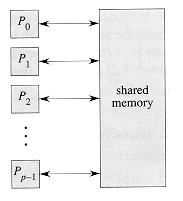
Figure 30.1 The basic architecture of the PRAM. There are p processors P0, P1, . . ., Pp - 1 connected to a shared memory. Each processor can access an arbitrary word of shared memory in unit time.
 EREW: exclusive read and exclusive write, CREW: concurrent read and exclusive write, ERCW: exclusive read and concurrent write, and CRCW: concurrent read and concurrent write. arbitrary: an arbitrary value from among those written is actually stored, priority: the value written by the lowest-indexed processor is stored, and combining: the value stored is some specified combination of the values written.
30.1 Pointer jumping
30.1.1 List ranking
 3,4,6,1,0,5
 . Since there is one processor per list object, every object in the list can be operated on by its responsible processor in O(1) time.
 (n) time, since the kth object from the end must wait for the k- 1 objects following it to determine their distances from the end before it can determine its own. This solution is essentially a serial algorithm.
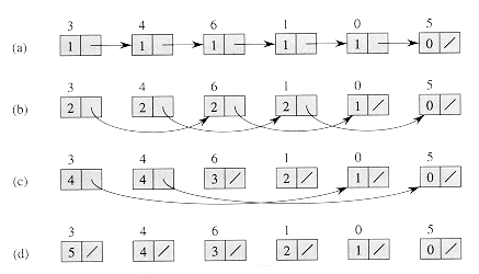
Figure 30.2 Finding the distance from each object in an n-object list to the end of the list in O(lg n) time using pointer jumping. (a) A linked list represented in a PRAM with d values initialized. At the end of the algorithm, each d value holds the distance of its object from the end of the list. Each object's responsible processor appears above the object. (b)-(d) The pointers and d values after each iteration of the while loop in the algorithm LIST-RANK.
LIST-RANK(L)
1 for each processor i, in parallel
2 do if next[i] = NIL
3 then d[i]
 0
04 else d[i]
15 while there exists an object i such that next[i]
 NIL
NIL6 do for each processor i, in parallel
7 do if next[i]
NIL8 then d[i]
d[i] + d[next[i]]9 next[i]
next[next[i]] next[next[i]] for all non-nil pointers next[i], is called pointer jumping. Note that th e pointer fields are changed by pointer jumping, thus destroying the structure of the list. If the list structure must be preserved, then we make copies of the next pointers and use the copies to compute the distances.Correctness
3,6,0 whose d values 2, 2, and 1 sum to 5, its distance from the end of the original list. The reason the invariant is maintained is that when each object "splices out" its successor in the list, it adds its successor's d value to its own. next[j] or next[i] = next[j] = NIL. This invariant is certainly true for the initial list, and it is maintained by line 9. Because all non-NIL next values are distinct, all reads in line 9 are exclusive. NIL and there is another object j pointing to i (that is, next[j] = i), then the first read fetches d[i] for processor i and the second read fetches d[i] for processor j. Thus, List-Rank is an EREW algorithm.Analysis
 lg n
lg n iterations. The key observation is that each step of pointer jumping transforms each list into two interleaved lists: one consisting of the objects in even positions and the other consisting of objects in odd positions. Thus, each pointer-jumping step doubles the number of lists and halves their lengths. By the end of lg n iterations, therefore, all lists contain only one object.(n lg n) work, since it requires n processors and runs in (lg n) time. The straightforward serial algorithm for the list-ranking problem runs in (n) time, indicating that more work is performed by List-Rank than is absolutely necessary, but only by a logarithmic factor.(n) time on a serial RAM, LIST-RANK is not work-efficient. We shall present a work-efficient parallel algorithm for list ranking in Section 30.4.
30.1.2 Parallel prefix on a list
 . The computation takes as input a sequence x1, x2, . . . , xn and produces as output a sequence y1, y, . . . , yn such that y1 = x1 and
yk = yk-1
xk= x1
x2 . . . xk be ordinary addition. Since the kth element of the list contains the value xk = 1 for k = 1,2, . . ., n, a prefix computation produces yk = k, the index of the kth element. Thus, another way to perform list ranking is to reverse the list (which can be done in O(1) time), perform this prefix computation, and subtract 1 from each value computed.[i, j] = xi
xi+1  xj
xj  i j n. Then, [k,k] = xk for
k = 1, 2,..., n, and
[i,k] = [i, j]
[j+1, k] i j < k n. In terms of this notation, the goal of a prefix computation is to compute yk = [1, k] for k = 1, 2, . . . , n.x1, x2, . . . , xn to be determined by how the objects are linked together in the list, and not by the index of the object in the array of memory that stores objects. (Exercise 30.1-2 asks for a prefix algorithm for arrays.) The following EREW algorithm starts with a value x[i] in each object i in a list L. If object i is the kth object from the beginning of the list, then x[i] = xk is the kth element of the input sequence. Thus, the parallel prefix computation produces y[i] = yk = [1, k].LIST-PREFIX(L)
1 for each processor i, in parallel
2 do y[i]
x[i]3 while there exists an object i such that next[i]
NIL4 do for each processor i, in parallel
5 do if next[i]
NIL6 then y[next[i]]
y[i] y[next[i]]7 next[i]
next[next[i]] next[j] or next[i] = next[j] = NIL. [k + 1, k + 1], yielding [k, k + 1], which it stores back into its successor. The next pointers are then jumped as in LIST-RANK, and the result of the first iteration appears in Figure 30.3(b). We can view the second iteration similarly. For k = 1, 2, . . . , n - 2, the kth object fetches the value [k + 1, k + 2] from its successor (as defined by the new value in its field next), and then it stores [k - 1, k] [k + 1, k + 2] = [k - 1, k + 2] into its successor. The result is shown in Figure 30.3(c). In the third and final iteration, only the first two list objects have non-NIL pointers, and they fetch values from their successors in their respective lists. The final result appears in Figure 30.3(d). The key observation that makes LIST-PREFIX work is that at each step, if we perform a prefix computation on each of the several existing lists, each object obtains its correct value.
Figure 30.3 The parallel prefix algorithm LIST-PREFIX on a linked list. (a) The initial y value of the kth object in the list is [k, k]. The next pointer of the kth object points to the (k + 1)st object, or NIL for the last object. (b)-(d) The y and next values before each test in line 3. The final answer is in part (d), in which the y value for the kth object is [1, k] for all k.
(n 1g n).30.1.3 The Euler-tour technique
(n) time--no better than the serial algorithm. Using the Euler-tour technique, however, we can compute node depths in O(lg n) time on an EREW PRAM, whatever the height of the tree. A node's A processor points to the A processor of its left child, if it exists, and otherwise to its own B processor. A node's B processor points to the A processor of its right child, if it exists, and otherwise to its own C processor. A node's C processor points to the B processor of its parent if it is a left child and to the C processor of its parent if it is a right child. The root's C processor points to NIL.
Figure 30.4 Using the Euler-tour technique to compute the depth of each node in a binary tree. (a) The Euler tour is a list corresponding to a walk of the tree. Each processor contains a number used by a parallel prefix computation to compute node depths. (b) The result of the parallel prefix computation on the linked list from (a). The C processor of each node (blackened) contains the node's depth. (You can verify the result of this prefix computation by computing it serially.)
Exercises
 n/2
n/2 th) object.
30.2 CRCW algorithms versus EREW algorithms
A problem in which concurrent reads help
FIND-ROOTS(F)
1. for each processor i, in parallel
2. do if parent[i] = NIL
3. then root[i]
i4. while there exists a node i such that parent[i]
NIL5. do for each processor i, in parallel
6. do if parent[i]
NIL7. then root[i]
root[parent[i]]8. parent[i]
parent[parent[i]] (lg n) time is required. The key observation is that when reads are exclusive, each step of the PRAM allows a given piece of information to be copied to at most one other memory location; thus the number of locations that can contain a given piece of information at most doubles with each step. Looking at a single tree, we have initially that at most 1 memory location stores the identity of the root. After 1 step, at most 2 locations can contain the identity of the root; after k steps, at most 2k-1 locations can contain the identity of the root. If the size of the tree is (n), we need (n) locations to contain the root's identity when the algorithm terminates; thus, (lg n) steps are required in all.(n) nodes, d = O(lg n), in which case FIND-ROOTS runs in O(lg lg n) time. Any EREW algorithm for this problem must run in (lg n) time, which is asymptotically slower. Thus, concurrent reads help for this problem. Exercise 30.2-1 gives a simpler scenario in which concurrent reads help.
Figure 30.5 Finding the roots in a forest of binary trees on a CREW PRAM. Node numbers are next to the nodes, and stored root fields appear within nodes. The links represent parent pointers. (a)-(d) The state of the trees in the forest each time line 4 of FIND-ROOTS is executed. Note that path lengths are halved in each iteration.
A problem in which concurrent writes help
(lg n) time and that no CREW algorithm does any better. The problem can be solved in O(1) time using a common-CRCW algorithm, in which when several processors write to the same location, they all write the same value. i, j n - 1. In effect, the algorithm performs a matrix of comparisons, and so we can view each of the n2 processors as having not only a one-dimensional index in the PRAM, but also a two-dimensional index (i, j).FAST-MAX(A)
1 n
length[A]2 for i
0 to n - 1, in parallel3 do m[i]
TRUE4 for i
0 to n -1 and j 0 to n - 1, in parallel5 do if A[i] < A[j]
6 then m[i]
FALSE7 for i
0 to n - 1, in parallel8 do if m[i] = TRUE
9 then max
A[i]10 return max
FALSE to record this fact. Several (i, j) pairs may be writing to m[i] simultaneously, but th ey all write the same value: FALSE.
Figure 30.6 Finding the maximum of n values in O(1) time by the CRCW algorithm FAST-MAX for each ordered pair of the elements in the input array A =
5, 6, 9, 2, 9, the result of the comparison A[i] < A[j] is shown in the matrix, abbreviated T for TRUE and F for FALSE. For any row that contains a TRUE value, the corresponding element of m, shown at the right, is set to FALSE. Elements of m that contain TRUE correspond to the maximum-valued elements of A. In this case, the value 9 is written into the variable max.(n)-time serial algorithm. We can come closer to a work-efficient algorithm, however, as Exercise 30.2-6 asks you to show. (lg n) time. The proof is conceptually similar to the lower-bound argument for finding the root of a binary tree. In that proof, we looked at how many nodes can "know" the identity of the root and showed that it at most doubles for each step. For the problem of computing the maximum of n elements, we consider how many elements "think" that they might possibly be the maximum. Intuitively, with each step of an EREW PRAM, this number can at most halve, which leads to the (lg n) lower bound.(lg n) lower bound for computing the maximum holds even if we permit concurrent reading; that is, it holds for CREW algorithms. Cook, Dwork, and Reischuk [50] show, in fact, that any CREW algorithm for finding the maximum of n elements must run in (lg n) time, even with an unlimited number of processors and unlimited memory. Their lower bound also holds for the problem of computing the AND of n boolean values.
Simulating a CRCW algorithm with an EREW algorithm

Figure 30.7 Simulating a concurrent write on an EREW PRAM. (a) A step of a common-CRCW algorithm in which 6 processors write concurrently to global memory. (b) Simulating the step on an EREW PRAM. First, ordered pairs containing location and data are written to an array A. The array is then sorted. By comparing adjacent elements in the array, we ensure that only the first of each group of identical writes into global memory is implemented. In this case, processors P0, P2, and P5 perform the write.
j, k p - 1. If lj lk or i = 0, then processor Pi, for i = 0, 1, . . . , p - 1, writes the datum xj to location lj in global memory. Otherwise, the processor does nothing. Since the array A is sorted by first coordinate, only one of the processors writing to any given location actually succeeds, and thus the write is exclusive. This process thus implements each step of concurrent writing in the common-CRCW model in O(lg p) time. Exercises
(lg n) time. n boolean matrices using n3 processors. n matrices of real numbers using n3 processors. Is there a faster common-CRCW algorithm? Is there a faster algorithm in one of the stronger CRCW models?
 > 0, there is an O(1)-time CRCW algorithm using O(n1+) processors to find the maximum element of an n-element array.
30.3 Brent's theorem and work efficiency

Figure 30.8 Brent's theorem. The combinational circuit of size 15 and depth 5 is simulated by a 2-processor CREW PRAM in 9
15/2 + 5 steps. The simulation proceeds from top to bottom through the circuit. The shaded groups of circuit elements indicate which elements are simulated at the same time, and each group is labeled with a number corresponding to the time step when its elements are simulated. ni/p groups, where the first ni/p groups have p elements each and the leftover elements, if any, are in the last group, the PRAM can simulate the computations performed by these combinational elements in O(ni/p) time. The total simulation time is therefore on the order of
 p/p' ). There are t steps, and so the entire simulation takes time O(p/p' t) = O(pt/p'), since p' < p. (w/t) processors in order to obtain work-efficient algorithms for all numbers of processors for which a work-efficient algorithm is possible. For p' = o(p), Theorem 30.4 guarantees that there is a work-efficient algorithm. For p' = w (p), no work-efficient algorithms exist, since if t is a lower bound on the time for any parallel algorithm, p't = w(pt) = w(w).
Exercises
n matrix A by an n-vector b in O(lg n) time with a work-efficient EREW algorithm. (Hint: Construct a combinational circuit for the problem.) n matrices. The algorithm should be work-efficient with respect to the normal (n3)-time serial algorithm for multiplying matrices. Can you make the algorithm EREW?* 30.4 Work-efficient parallel prefix computation
(n lg n) work. Since we can easily perform a prefix computation in (n) time on a serial machine, LIST-RANK is not work-efficient.(n/lg n) processors, and it runs in O(lg n) time with high probability. Thus, it is work-efficient with high probability. Moreover, by Theorem 30.4, this algorithm immediately yields work-efficient algorithms for any number p = O(n/lg n) of processors.Recursive parallel prefix computation
(n/ lg n) processors. During the algorithm, each processor is responsible for n/p = (lg n) of the objects in the original list. The objects are assigned to processors arbitrarily (not necessarily contiguously) before the recursion begins, and "ownership" of objects never changes. For convenience, we assume that the list is doubly linked, since doubly linking a single list takes O(1) time. [k + 1, k + 1]. The kth object is then eliminated from the list by splicing it out.
Figure 30.9 The work-efficient, randomized, recursive, parallel algorithm RANDOMIZED-LIST-PREFIX for performing prefix computations on a linked list of n = 9 objects. (a)-(b) A set of nonadjacent objects (blackened) are selected for elimination. The value in each black object is used to update the value in the next object in the list, and then the black object is spliced out. The algorithm is called recursively to compute a parallel prefix on the contracted list. (c)-(d) The resulting values are the correct final values for objects in the contracted list. The eliminated objects are then spliced back in, and each uses the value of the previous object to compute its final value.
[k, k].
Figure 30.10 The recursive stages of RANDOMIZED-LIST-PREFIX, shown for n = 9 original objects. In each stage, the blackened objects are eliminated. The procedure recurses until the list is empty, and then the eliminated objects are spliced back in.
Selecting objects for elimination
Analysis
(lg n) objects, the expected time for a processor to eliminate all its objects is (lg n).(1g n). For example, if most of the processors eliminate all their objects quickly and a few processors take much, much longer, the average time for a processor to eliminate all its objects might still be (lg n), but the running time of the algorithm could be large.(lg n), even though the simple analysis does not show it. We shall use a high-probability argument to prove that with probability at least 1 - 1/n, all objects are eliminated within c lg n stages of the recursion, for some constant c. Exercises 30.4-4 and 30.4-5 ask you to generalize this argument to prove the (lg n) bound on the expected running time.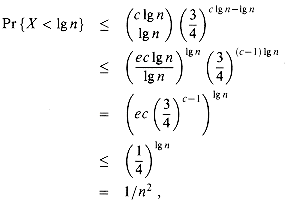
 20. (The second line follows from inequality (6.9).) Thus, the probability that all objects belonging to a given processor have not been eliminated after c lg n steps is at most 1/n2.
 20 in the c 1g n running time may seem a bit large for practicality. In fact, this constant is more an artifact of the analysis than a reflection of the algorithm's performance. In practice, the algorithm tends to be fast. The constant factors in the analysis are large because the event that one processor finishes eliminating all its list objects is dependent on the event that another processor finishes all its work. Because of these dependencies, we used Boole's inequality, which does not require independence but results in a weaker constant than would generally be experienced in practice.
Exercises
1, RANDOMIZED-LIST-PREFIX runs in O(lg n) time with probability at least 1 - 1/nk. Show how the constant in the running-time bound is influenced by k.30.5 Deterministic symmetry breaking
5 for all n 265536, the value lg* n can be viewed as a small constant for all practical purposes (see page 36).Colorings and maximal independent sets
 N such that for all u, v V, if C(u) = C(v), then (u, v)
  E; that is, no adjacent vertices have the same color. In a 6-coloring of a linked list, all colors are in the range {0, 1, 2, 3, 4, 5} and no two consecutive vertices have the same color. In fact, any linked list has a 2-coloring, since we can color objects whose ranks are odd with color 0 and objects whose ranks are even with color 1. We can compute such a coloring in O(lg n) time using a parallel prefix computation, but for many applications, it suffices to compute only an O(1)-coloring. We shall show that a 6-coloring can be computed in O(lg* n) time without using randomization.
 V of vertices such that each edge in E is incident on at most one vertex in V'. A maximal independent set, or MIS, is an independent set V' such that for all vertices v V - V', the set V'
  {v} is not independent--every vertex not in V' is adjacent to some vertex in V'. Do not confuse the problem of computing a maximal independent set--an easy problem--with the problem of computing a maximum independent set--a hard problem. The problem of finding an independent set of maximum size in a general graph is NP-complete. (See Chapter 36 for a discussion of NP-completeness. Problem 36-1 concerns maximum independent sets.)n/2 objects. Observe, however, that any maximal independent set of a linked list contains at least n/3 objects, since for any 3 consecutive objects, at least one must be in the set. We shall show, however, that a maximal independent set of a list can be determined in O(1) time given an O(1)-coloring of the list.
Computing a 6-coloring
{0, 1, . . . , n - 1}.lg n bits, which means that it can be stored in an ordinary computer word.ar-1, ar-2, . . . , a0 and b = br-1, br-2, . . . , b0 are r-bit colors. Since Ck[x] Ck[next[x]], there is some least index i at which the bits of the two colors differ: ai bi. Because 0 i r - 1, we can write i with only [lg r] bits: i = i lg r-1, ilg r-2, . . . , i0. We recolor x with the value of i concatenated with the bit ai. That is, we assignCk+1[x] =
i, ai=
ilg r - 1, i lg r-2, . . . , i0, ai.lg r + 1. Ck next[x]] implies Ck+1[x] Ck+1[next[x]]. Suppose that Ck[x] = a and Ck[next[x]] = b, and that Ck+1[x] = i, ai and Ck+1[next[x]] = j, bj. There are two cases to consider. If i j, then i, ai j, bj, and so the new colors are different. If i = j, however, then ai bi = bj by our recoloring method, and thus the new colors are once again different. (The situation at the tail of the list can be handled similarly.)lg r + 1)-bit color, which means that the number of bits is strictly reduced as long as r 4. When r = 3, two colors can differ in bit position 0, 1, or 2. Each new color, therefore, is 00, 01, or 10 concatenated with either 0 or 1, thus leaving a 3-bit number once again. Only 6 of the 8 possible values for 3-bit numbers are used, however, so that SIX-COLOR indeed terminates with a 6-coloring.
Figure 30.11 The algorthms SIX-COLOR and LIST-MIS that break symmetry in a list. Together, the algorithms find a large set of nonadjacent objects in O(lg* n) time using n processors. The initial list of n = 20 objects is shown on the left, running vertically. Each object has an initial, distinct 5-bit color. For these parameters, the algorithm SIX-COLOR needs only the two iterations shown to recolor each object with a color in the range {0, 1, 2, 3, 4, 5}. White objects are placed into the MIS by LIST-MIS as the colors are processed, and black objects are killed.
lg* n = min {i 0 : lg(i) n 1} .lg(i) n 2, then ri lg(i) n + 2. Initially, we have r1 lg n. The ith iteration brings the number of bits in the coloring down to ri+1 = lg ri + 1. Assuming that the inductive hypothesis holds for ri - 1, we obtainri =
lg ri-1 + 1 lg(lg(i-1)n + 2) + 1 lg(lg(i-1)n + 3) + 1 lg(2 lg(i-1)n) + 1=
lg(lg(i-1)n) + 1 + 1=
lg (i)n + 2.lg(i) n 2, which means that lg(i-1)n 3. Therefore, after m = lg* n steps, the number of bits in the coloring is rm lg(m) n + 2 = 3, since lg (m) n 1 by defination of the lg* function. Thus, at most one more iteration suffices to produce a 6-coloring. The total time of SIX-COLOR is therefore O(lg* n).Computing an MIS from a 6-coloring
C[next[x]], because C is a coloring. Without loss of generality, we assume that C[x] < C[next[x]], so that x is placed into the set before next[x] is. But then alive[next[x]] has been set to FALSE by the time objects of color C[next[x]] are considered, and next[x] could not have been place into the set.Exercises
Problems
. It takes an input sequence x = x1, x2, . . . , xn whose elements are drawn from a domains and a segment sequence b = b1, b2, . . . , bn whose elements are drawn from the domain {0,1}, with b1 = 1. It produces an output sequence y = y1, y2, . . . , yn over the domain S. The bits of b determine a partitioning of x and y into segments; a new segment begins wherever bi = 1, and the current one continues if bi = 0. The segmented prefix computation performs an independent prefix computation within each segment of x to produce the corresponding segment of y. Figure 30.12 illustrates a segmented prefix computation using ordinary addition. on ordered pairs (a, z), (a', z') {0, 1} X S as follows:
 is associative. p/2 numbers can be reduced to the problem of finding the maximum of at most m2/p numbers in O(1) time on a p-processor CRCW PRAM.p/2 numbers, how many numbers remain after k iterations of the algorithm in part (a)?
Figure 30.12 A segmented prefix computation with segment sequence b, input sequence x, and output sequence y. There are 5 segments.
V maintains a pointer p[v] to a parent. Initially, p[v] = v: the vertex points to itself. At the end of the algorithm, for any two vertices u, v V, we have p[u] = p[v] if and only if  in G. During the algorithm, the p pointers form a forest of rooted pointer trees. A star is a pointer tree in which p[u] = p[v] for all vertices u and v in the tree. E appears twice: once as (u,v) and once as (v,u). The algorithm uses two basic operations, HOOK and JUMP, and a subroutine STAR that sets star[v] = TRUE if v belongs to a star.
HOOK(G)
1 STAR (G)
2 for each edge (u, v)
E[G], in parallel3 do if star[u] and p[u] > p[v]
4 then p[p[u]]
p[v]5 STAR(G)
6 for each edge (u, v)
E[G], in parallel7 do if star[u] and p[u]
p[v]8 then p[p[u]]
p[v]JUMP(G)
1 for each v
V[G], in parallel2 do p[v]
p[p[v]] in G.
in G. in G.
in G.
 (C) by a constant factor.(C) |V|.(C).(C) is at most 2/3 its previous value. Illustrate the worst case.
M[r2 + i, c2 + j]
M[r2 + i, c2 + j] * M[r1 + i, c1 + j] M[j, i]) in the visible portion of the frame buffer. We assume that the cost of copying the bits is less than that of calling the BITBLT primitive, and hence we are interested in using as few BITBLT operations as possible.Chapter notes
(lg n) time on a CREW PRAM. The simulation of a CRCW algorithm with an EREW algorithm is due to Vishkin [195].