|
Nighttime Haze Removal with Illumination Correction
Jing Zhang Student Member, IEEE, Yang Cao Member, IEEE, Zengfu Wang Member, IEEE
|
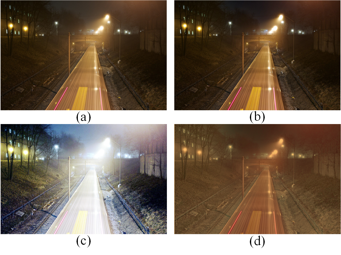
Fig. 1. (a) A nighttime haze image. (b) Dehazing reuslt of [10]. (c) Histogram equalization result. (d) Result of [12].
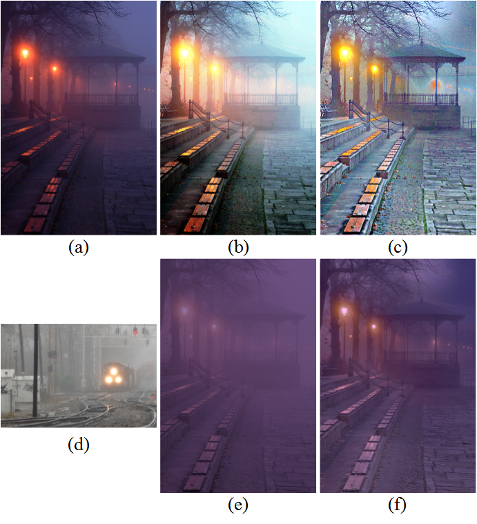
Fig. 2. (a) A nighttime haze image. (b) Histogram equalization result. (c) Result of the proposed algorithm. (d) A daytime haze image used as the target image in [12]. (e) Statistic correction result of [12]. (f) Final dehazing result of [12].

Fig. 3. (a) A daytime haze image. (b) Dehazing result of [7]. (c) Dehazing result of [11].
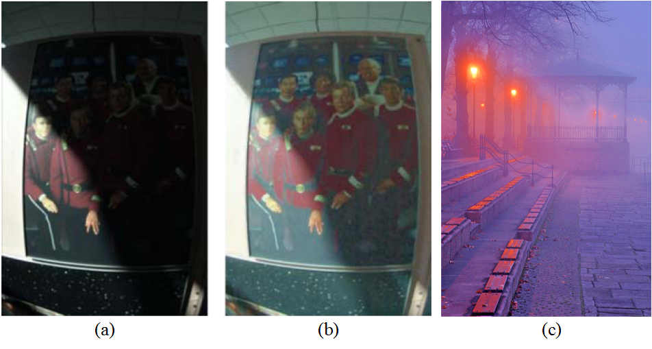
Fig. 4. (a) An illumination unbalanced image. (b) Result of (a) by using method in [15]. (c) Result of Fig. 2(a) by using method in [15].

Fig. 5. (a) Some examples of clear daytime images. (b) Statistics of illumination intensities of clear and nighttime haze images. (c) Some examples of nighttime haze images. (d) Statistics of standard deviations of values on local patches.
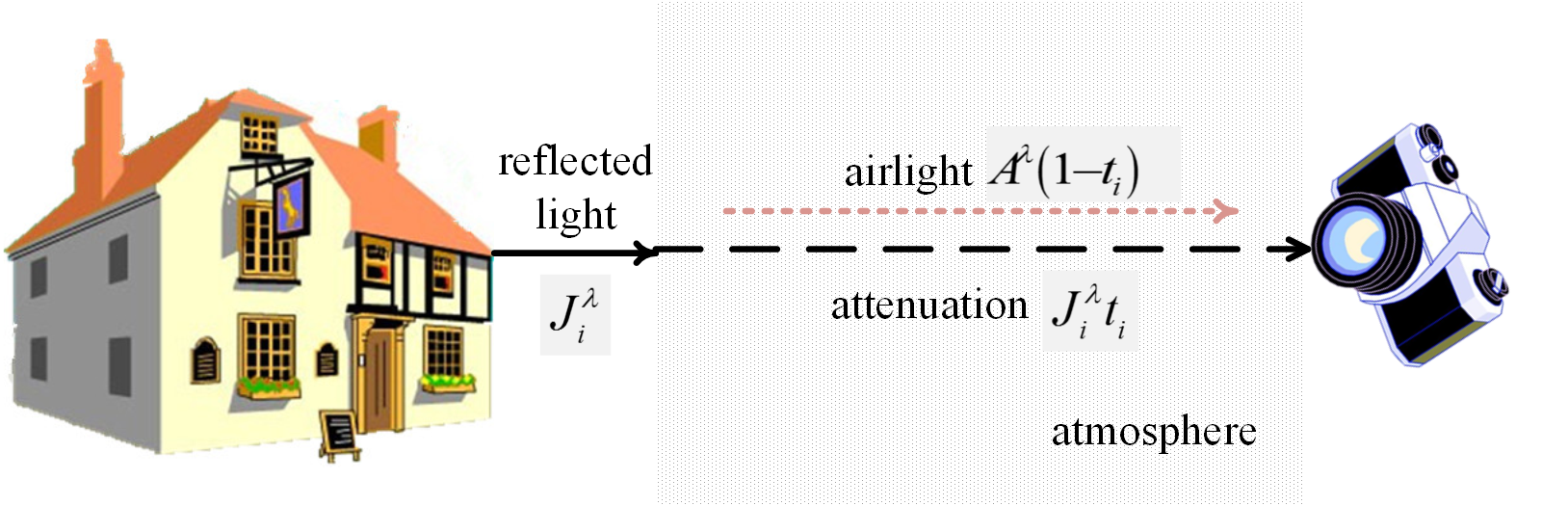
Fig. 6. A macro physical picture of the daytime haze imaging model. It is replotted from Fig.2.2 in [9].
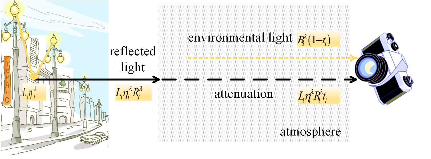
Fig. 7. A macro physical picture of the nighttime haze imaging model.
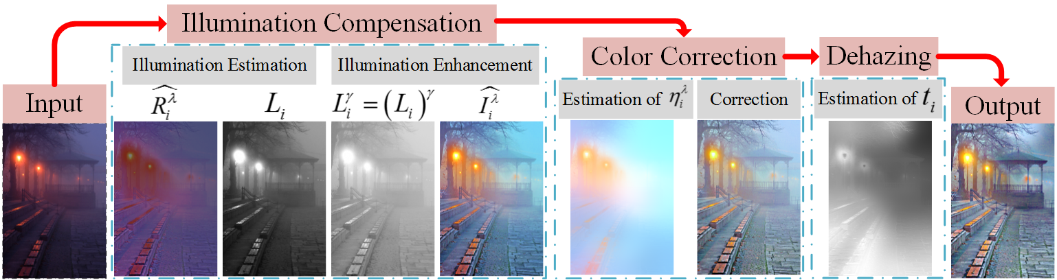
Fig. 8. A diagram of the proposed algorithm.
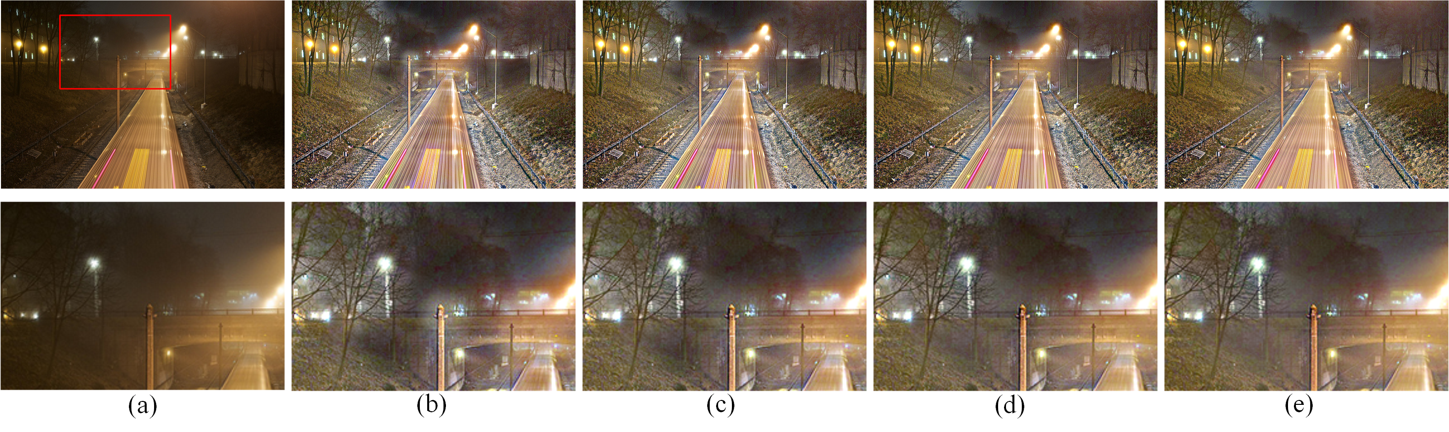
Fig. 9. Comparisons on different settings of kernel size of image guided filter. (a) Input nighttime haze image and the close-up view of the redbox region. (b)-(e) show the results of the proposed algorithm and the close-up views by setting different kernel sizes of image guided filter. The kernel radius of image guided filter is set to 8, 16, 32 and 64 in (b)-(e), respectively.

Fig. 10. Comparisons on different settings of local patch sizes when estimating ¦Ç^¦Ë_i and A^¦Ë_i. (a)-(e) show the results of the proposed algorithm and the close-up views by setting different local patch sizes. The radius of local patch is set to 3, 5, 7, 9 and 11 in (a)-(e), respectively.

Fig. 11. (a) Original nighttime haze images. (b) Retinex results of [15]. (c) Results of Histogram equalization. (d) Results of He et al.¡¯s method [10]. (e) Results of Pei et al.¡¯s method [12]. (f) Results of the proposed algorithm.
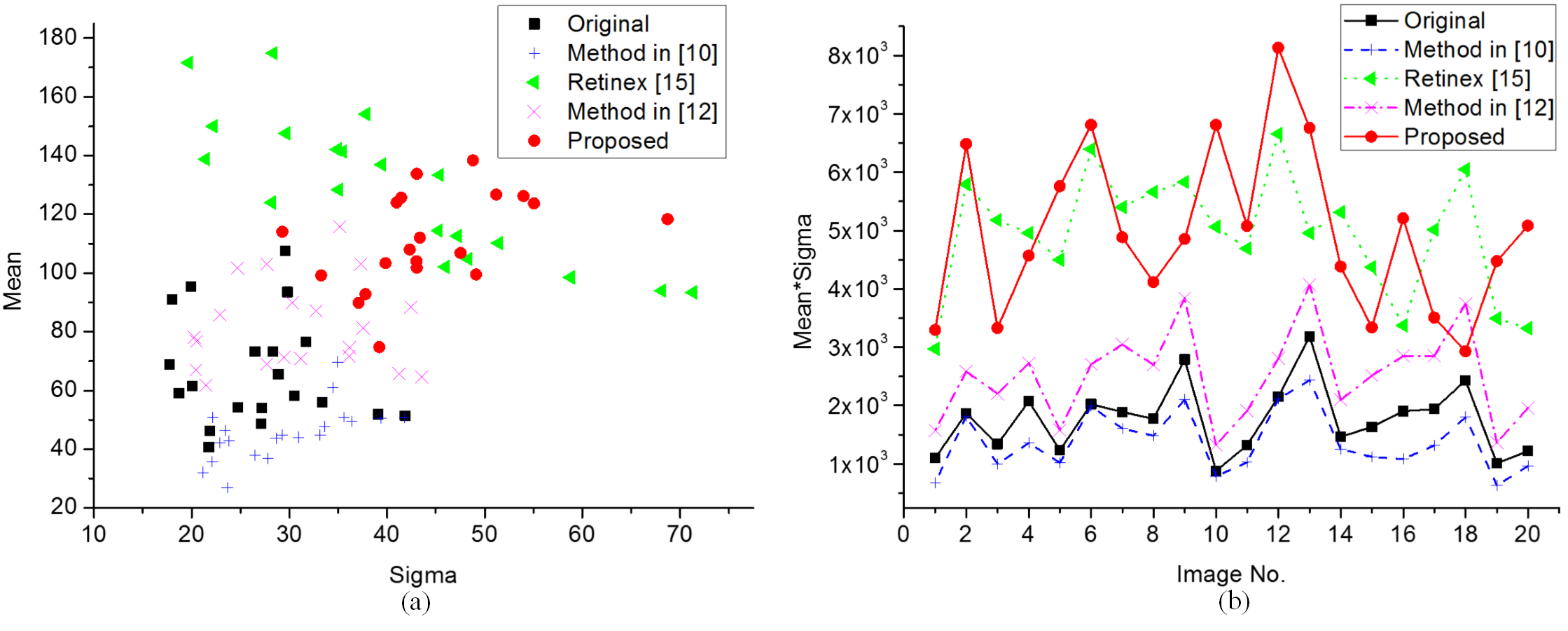
Fig. 12. (a) I and ¦̉ of results obtained by different methods on the 20 test images. (b) Visual measures of results obtained by different methods on the 20 test images.

Fig. 13. Color rendition experiment on color set images captured in nighttime haze environment. (a) Original nighttime haze images. (b) Results of He et
al.¡¯s method [10]. (c) Results of retinex method [15]. (d) Results of Pei et al.¡¯s method [12]. (e) Results of the proposed algorithm.
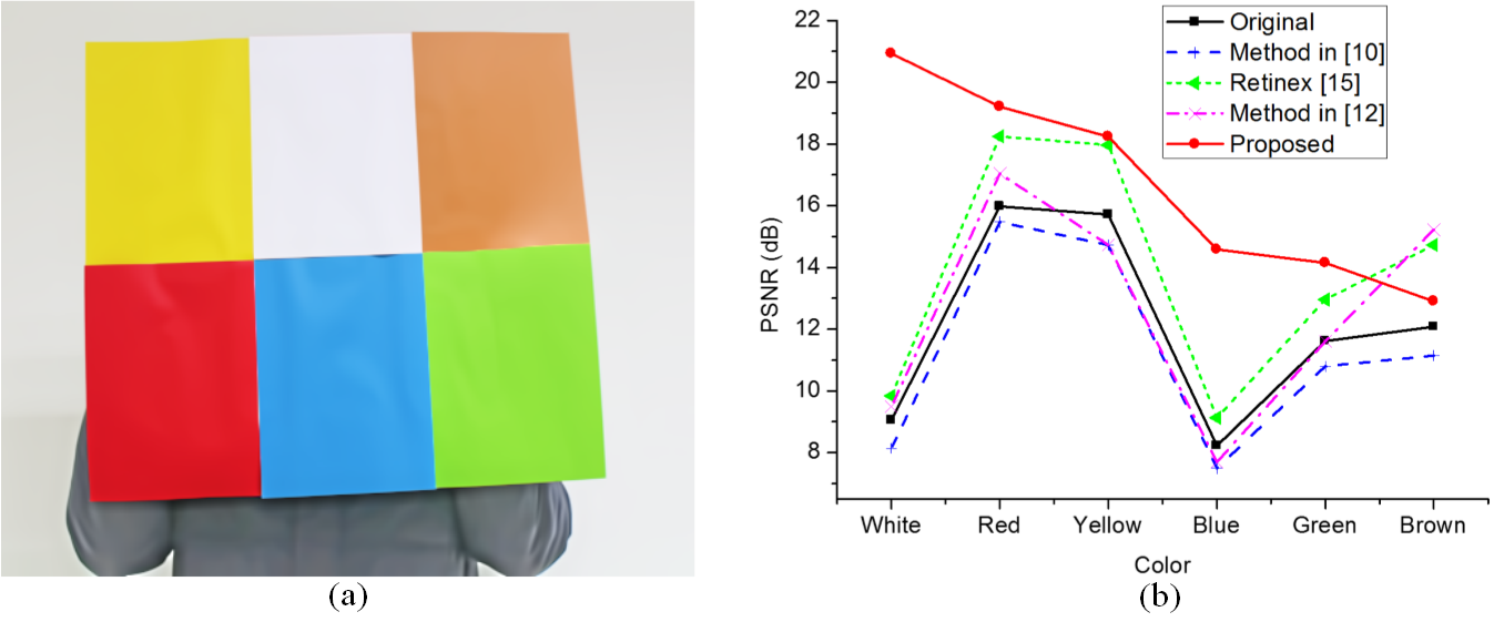
Fig. 14. (a) Ground truth color set captured in indoor environment with daylight lamp. (b) PSNRs of different methods on the six colors.
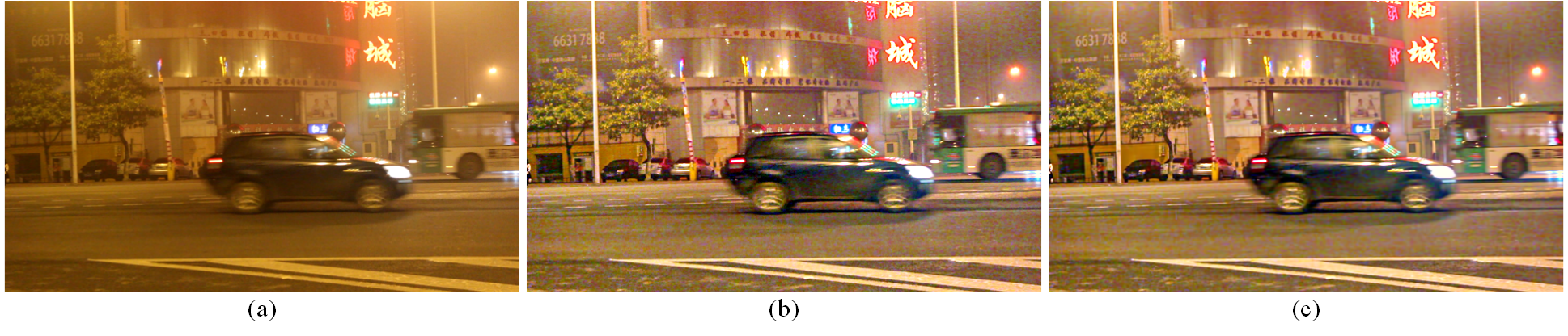
Fig. 15. (a) The 150^th frame of the test video sequence captured in nighttime haze environment. (b) Result of the proposed algorithm. (c) Denoising result of (b) by using BM3D denoising method [22].
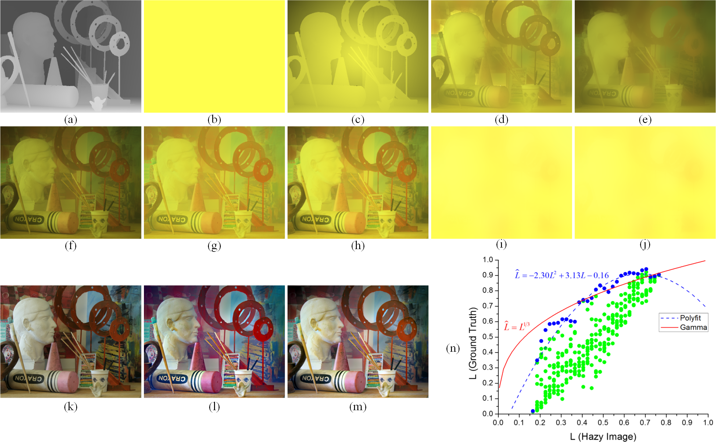
Fig. 16. Synthetic results on test image of ¡°Art¡±. (a) Disparity map. (b) color of light source, i.e., ¦Ç^¦Ë. (c) Illumination image. (d) Color of environmental light, i.e., ¦̉^¦Ë. (e) Environmental light image. (f) Synthetic nighttime hazy image. (g)-(h) Illumination compensation result of gamma correction and polynomial fitting. (i)-(j) Estimates of ¦Ç^¦Ë on (g)-(h). (k) Ground truth. (l)-(m) Final dehazing results by using gamma correction and polynomial fitting in the proposed algorithm, respectively. (n) Gamma curve and polynomial fitting curve about points on the upper bound.
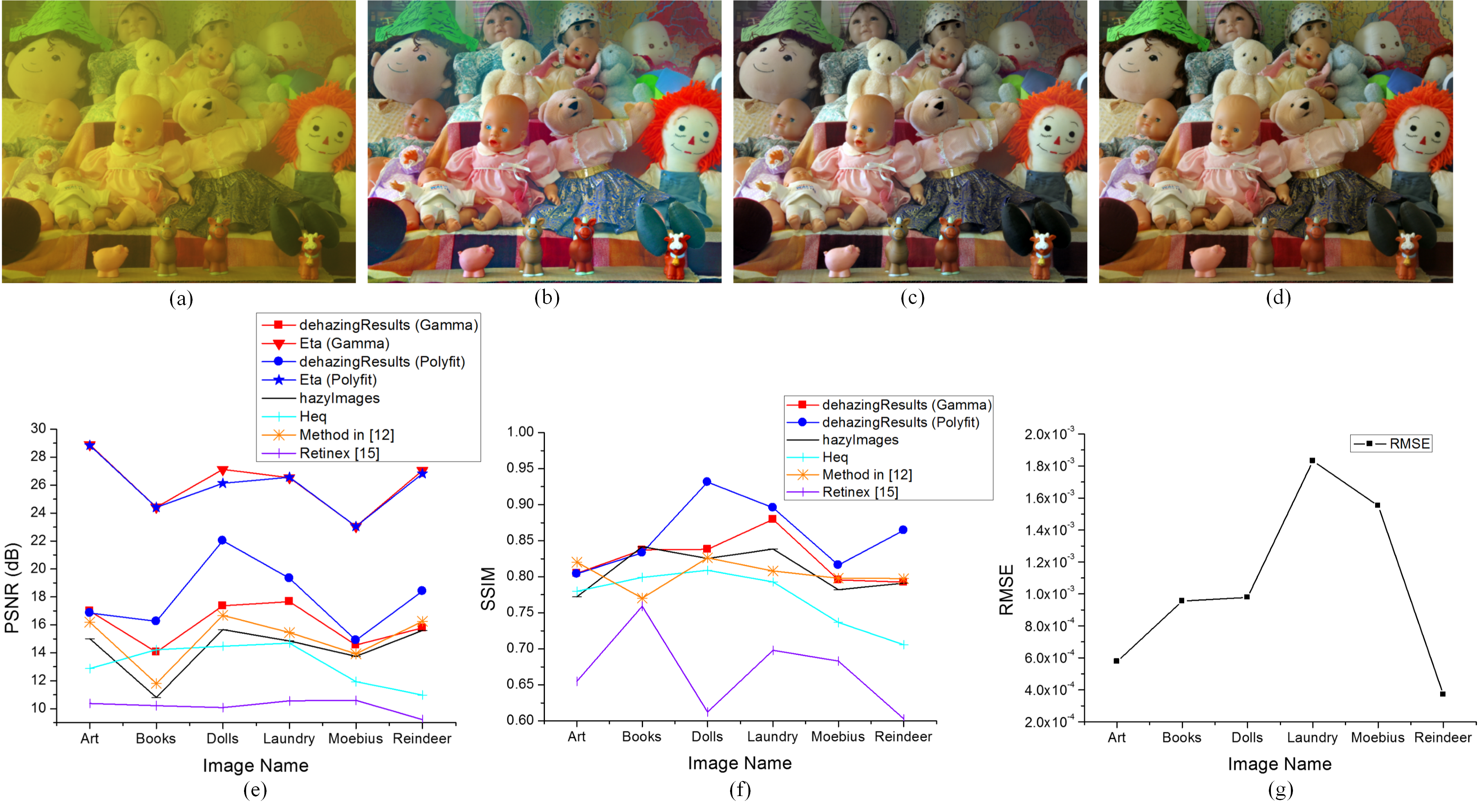
Fig. 17. (a) Synthetic nighttime hazy image of ¡°Dolls¡±. (b)-(c) Final dehazing reuslts by using gamma correction and polynomial fitting in the proposed
algorithm, respectively. (d) Ground truth. (e) PSNR indices of dehzing reuslts and estimates of ¦Ç^¦Ë. (f) SSIM indices of dehazing results. (e) RMSE between ¦Ç^¦Ë and max{¦Ç^¦Ë,¦̉^¦Ë}.
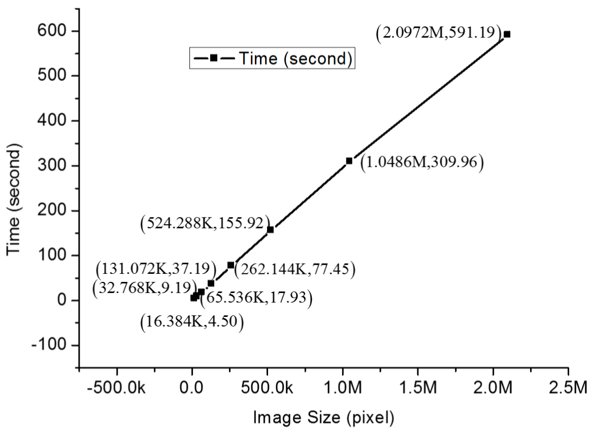
Fig. 18. Computation time v.s. image size.