Introduction
Bloch oscillation is a phenomenon from solid state physics. It describes the oscillation, both in real- and momentum-space, of a particle (e.g. an electron) confined in a periodic potential when a constant force is acting on it.1 In the current post, we will show the 1D Bloch oscillation using a simple 1D model periodic potential:
\[\begin{equation} V(x) = 2 v_0 \cos(\frac{2\pi}{a} x) \label{eq:1d_cosx_pot} \end{equation}\]where $a$ is the 1D periodicity and $v_0$ represents the strength of the potential. The Schrödinger equation for the electron in this model periodic potential reads
\[\begin{equation} \left[ -\frac{\hbar^2}{2m} \frac{\partial^2}{\partial x^2} + V(x) \right] \psi_{nk}(x) = \epsilon_{nk} \, \psi_{nk}(x) \label{eq:1d_schro_eq} \end{equation}\]where according to the Bloch theorem, the wavefunction takes the form of a Bloch wave.
\[\begin{equation} \psi_{nk}(x) = e^{ik\cdot x} u_{nk}(x) \label{eq:bloch_wave} \end{equation}\]Substituting Eq.\eqref{eq:bloch_wave} back to Eq.\eqref{eq:1d_schro_eq}, one can get the equation for the periodic part of the Bloch wave:
\[\begin{equation} \left[ \frac{\hbar^2}{2m} (-i\frac{\partial}{\partial x}+k)^2 + V(x) \right] u_{nk}(x) = \epsilon_{nk} \, u_{nk}(x) \label{eq:1d_unk_schro_eq} \end{equation}\]By expanding the periodic part $u_{nk}(x)$ using plane-waves $e^{iG\cdot x}$, i.e.
\[\begin{equation} u_{nk}(x) = \sum_G C(G) e^{iG\cdot x} \qquad (G = \frac{2n\pi}{a}, n\in\mathbb{N}) \end{equation}\]one obtains the central equation2
\[\begin{equation} \bigl[ \frac{ \hbar^2(\mathbf{k} + \mathbf{G}')^2 }{2m} - \epsilon_{n\mathbf{k}} \bigr] C(\mathbf{G}') \, \delta_{\mathbf{G},\mathbf{G}'} + \sum_{\mathbf{G}'} U_{\mathbf{G},\mathbf{G}'} C(\mathbf{G}') = 0 \label{eq:central_equation} \end{equation}\]where $U(G,G’)$ is the Fourier transform of the potential $V(x)$,
\[\begin{equation} U(\mathbf{G} - \mathbf{G}') = \int\, e^{-i(\mathbf{G} - \mathbf{G}')\cdot \mathbf{r}} V(\mathbf{r}) \,\mathrm{d}\mathbf{r} = \int\, e^{-i\mathbf{G}\cdot \mathbf{r}} V(\mathbf{r}) e^{i \mathbf{G}'\cdot \mathbf{r}} \,\mathrm{d}\mathbf{r} \equiv U_{\mathbf{G},\mathbf{G}'} \label{eq:central_eq_matrix} \end{equation}\]The central equation can also be written in the matrix form:
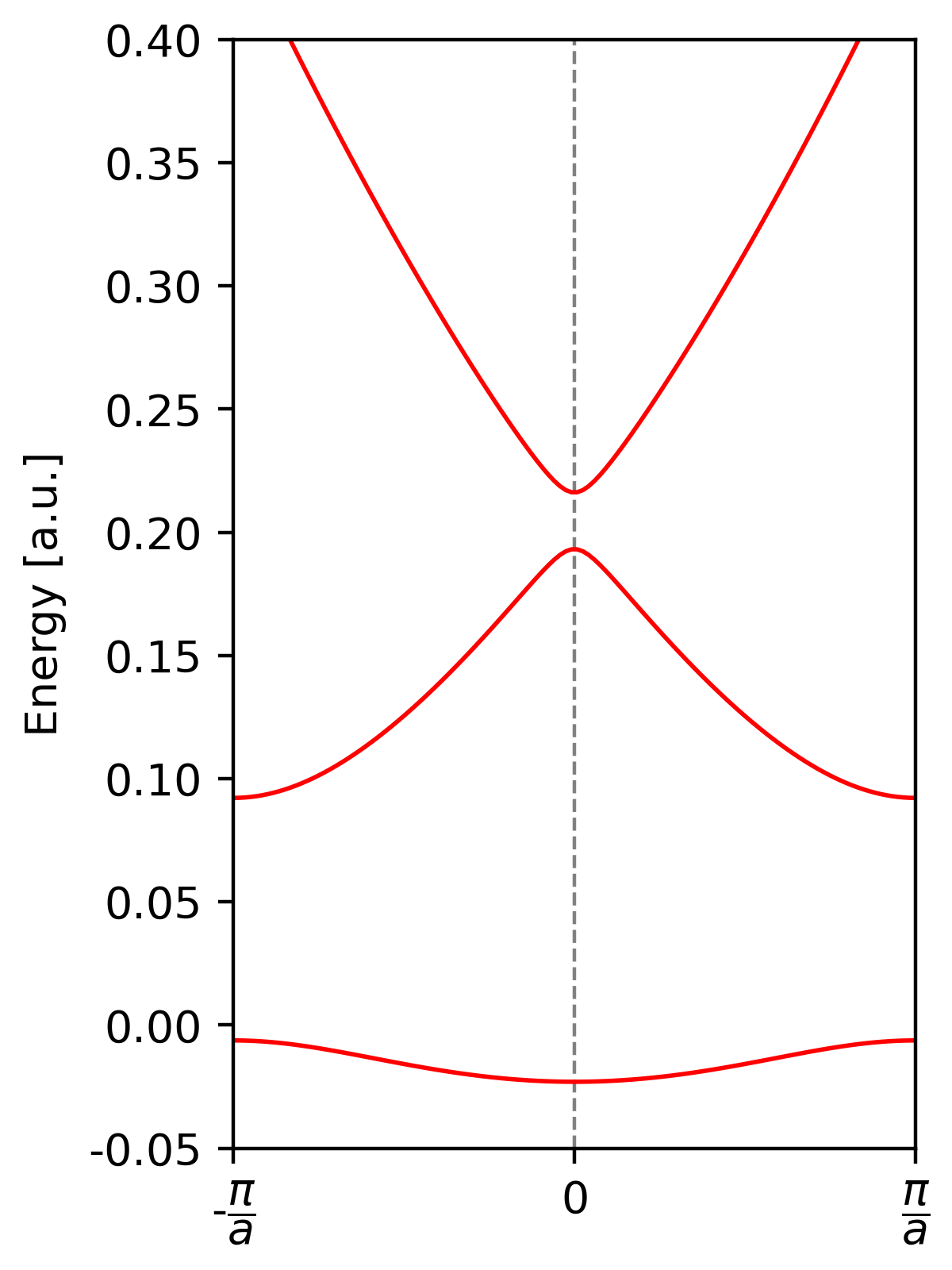
\[\begin{equation} \begin{bmatrix} \ddots & \vdots & \vdots & \vdots & \vdots\\[3pt] \vdots & \frac{\hbar^2(\mathbf{k}-G)^2}{2m} - \epsilon_{n\mathbf{k}} & U_{-G,0} & U_{-G,G} & \vdots\\[3pt] \vdots & U_{0,-G} & \frac{\hbar^2\mathbf{k}^2}{2m} - \epsilon_{n\mathbf{k}} & U_{0,G} & \vdots \\[3pt] \vdots & U_{G,-G} & U_{G,0} & \frac{\hbar^2(\mathbf{k}+G)^2}{2m} - \epsilon_{n\mathbf{k}} & \vdots\\[3pt] \vdots & \vdots & \vdots & \vdots & \ddots \end{bmatrix} \begin{bmatrix} \vdots \\[6pt] C_{-G} \\[6pt] C_{0} \\[6pt] C_{G} \\[6pt] \vdots \end{bmatrix} = 0 \end{equation}\]Band structure from the central equation
Construction of the Bloch wavepacket
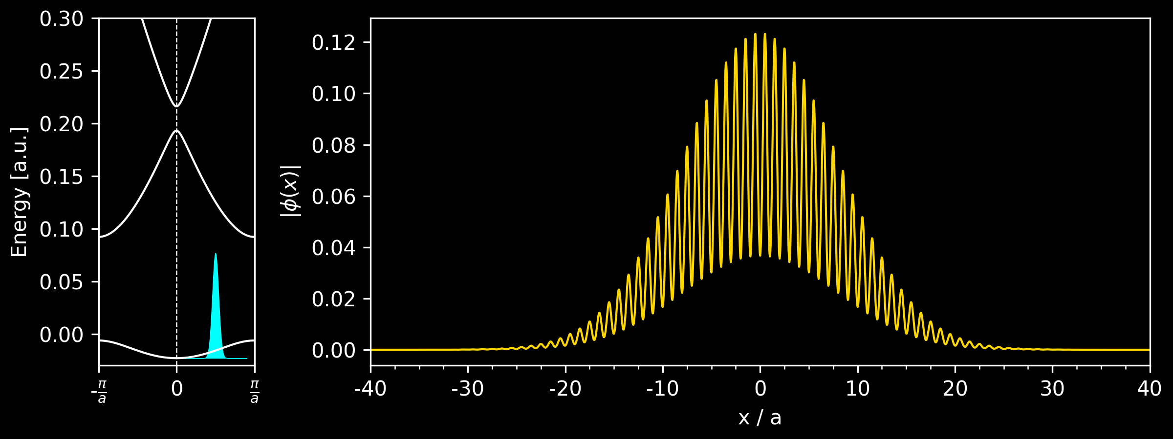
Next, we construct the Bloch wavepacket from the Bloch states
\[\begin{equation} w(x, k_c) = \sum_k F(k - k_c) \, \psi_{nk}(x) \end{equation}\]Here, we choose the Gaussian function as the envelope function for the Bloch wavepackets, i.e.
\[\begin{equation} F(k - k_c) = \frac{1}{\sqrt{2\pi}\sigma_k} e^{-\frac{(k-k_c)^2}{2\sigma_k^2}} \end{equation}\]where $k_c$ is the central momentum and $\sigma_k$ represents the spread of the Bloch wavepacket. Within the semiclassical model, it is required that $\sigma_k$ is much smaller than the size of the Brillouin zone.
Time evolution of the Bloch wavepacket
With the Bloch wavepacket as the initial wavefunction, we now consider the dynamics of the wavepacket under a constant external field, e.g. an electric field $E$. The time-dependent Schrödinger equation (TDSE) reads
\[\begin{equation} i\hbar \frac{\partial }{\partial t} w(x, k_c) = \left[ -\frac{\hbar^2}{2m}\nabla^2 + V(x) - qE x \right] w(x, k_c) \label{eq:tdse_efield} \end{equation}\]For the numerical solution of Eq.\eqref{eq:tdse_efield}, please refer to my previous post.3 The results are shown below, where one can clearly see that the average position $x_c$ and momentum $k_c$ of the Bloch wavepacket indeed oscillate with time.
