Angular Momentum in Solids

Conservation of Crystal Total Angular Momentum

Einstein-De Haas Effect

The Einstein–de Haas effect is a physical phenomenon in which a change in the magnetization causes mechanical rotation of the body. The effect is a consequence of the conservation of total angular momentum. ¹

Barnett Effect

The opposite effect of Einstein-De Hass effect is the Barnett effect — a change in rotation causes a magnetization. ²

Total Angular Momentum

In 2014, Niu et al.³ proposed that the total angular momentum for a crystal with non-zero phonon angular momentum consists of the following parts:

where

• ${\cal L}^\mathrm{lat}$ is the mechanical rotation of the whole crystal

• ${\cal L}^\mathrm{spin}$ is the spin angular momentum (SAM)

• ${\cal L}^\mathrm{orb}$ is the total orbital angular momentum (OAM)

• ${\cal L}^\mathrm{ph}$ is the total phonon angular momentum (PAM)

Traditionally, only the first three terms are considered in angular momentum conservation.

Phonon Angular Momentum

When the atoms of a crystal move along the path of a circularly polarized phonon mode, they form closed loops and therefore carry angular momentum. Below, we show animations of two typical phonon modes of graphene that involves circular motions.

Phonon angular momentum therefore refers to orbital motion of an atom in a lattice about its equilibrium position, and it can be likened to an electron’s orbital about the atomic center. In 2014, Niu et al. in their paper ³ first proposed to define the PAM as

where $\mathbf{u}^l_j$ is the displacement vector of the j-th atom in the P-th unit cell, multiplied by square root of mass $m_j$. After expressing the displacement vector in the second quantization form, they obtained the form of the total phonon angular momentum per unit cell if the system is in equilibrium

The summation (integration) is over all the phonon modes $\nu$ and phonon wavevectors $\mathbf{q}$ within the first Brillouin zone. In Eq\eqref{eq:total_pam}, $n_0(\omega_{\mathbf{q}\nu})$ is the Bose distribution for the $\nu$-th phonon mode at wavevector $\mathbf{q}$ with frequency $\omega_{\mathbf{q},\nu}$.

$l_{\mathbf{q},\nu}$ is the mode-decomposed phonon angular momentum

where the matrix $M_\alpha$ is the tensor product of the unit matrix and the generator of SO(3) rotation for a unit cell with N atoms ⁴

where $\varepsilon_{\alpha\beta\gamma}$ is the Levi-Civita epsilon tensor. ⁵

• For system with time-reversal symmetry (no magnetic field, not ferromagnets or anti-ferromagnets et al.), it can be proved that (See Supporting Information of Ref ³)

  \[\begin{equation} l_{-\mathbf{q},\nu}^\alpha = - l_{\mathbf{q},\nu}^\alpha \label{eq:zero_pam_sym} \end{equation}\]

  As a result, the sum in Eq.\eqref{eq:total_pam} is zero, i.e. the total phonon angular momentum is zero in equlibrium if the time-reversal symmetry is preserved (no spin-phonon interaction).

  Nevertheless, Murakami et al.⁴ showed that when a temperature gradient is applied and heat current flows in the crystal, the phonon distribution therefore becomes off-equilibrium, a finite angular momentum is then generated. There is also a report of temperature gradient induced transverse flow of PAM, the so-called phonon angular momentum Hall effect (PAMHE). ⁶

• At zero temperature, Eq.\eqref{eq:total_pam} reduces to

  \[\begin{equation} {\cal L}_\alpha^\mathrm{ph} = \sum_{\mathbf{q},\nu} \frac{1}{2} l_{\mathbf{q}\nu}^\alpha \label{eq:total_zero_pam} \end{equation}\]

  This means that each phonon mode has a zero-point angular momentum $\frac{1}{2}l_{\mathbf{q}\nu}$ in addition to a zero-point energy of $\frac{1}{2}\hbar\omega_{\mathbf{q}\nu}$.

• As the temperature increases, the total phonon angular momentum diminishes and approaches zero in the classical limit. ³

  \[\begin{equation} {\cal L}_\alpha^\mathrm{ph}(T \to \infty) = \sum_{\mathbf{q}\nu} \frac{ \hbar\omega_{\mathbf{q}\nu} }{12k_B T} \,l_{\mathbf{q}\nu}^\alpha \to 0 \end{equation}\]

Python Code Implementation

For brevity’s sake, let us assume $\alpha=z$, $\beta=x$ and $\gamma=y$ in Eq.\eqref{eq:mode_pam} and Eq.\eqref{eq:M_mat}. Then, $l_{\mathbf{q}\nu}^z$ can be written as

In the above equation $\boldsymbol\epsilon_{j,\mathbf{q}\nu}^{x}$ is the x-component of the phonon polarization vector from the j-th atom within the unit cell.

Similarly, one can have

• Eq.\eqref{eq:pam_z}, Eq.\eqref{eq:pam_x} and Eq.\eqref{eq:pam_y} can be combined and written in a much concise form:

  \[\begin{equation} l_{\mathbf{q}\nu} = -i\hbar \sum_j \boldsymbol\epsilon_{j,\mathbf{q}\nu}^* \times \boldsymbol\epsilon_{j,\mathbf{q}\nu} \label{eq:pam_oprod_form} \end{equation}\]

  For system with time-reversal symmetry (no magnetic field, not ferromagnets or anti-ferromagnets, no geometric phase et al.), the polarization vector $\boldsymbol\epsilon_{\mathbf{q}\nu}$ of the phonon modes at $\Gamma$ point can be chosen as real (up to a global irrelevant phase factor), as a result the phonon angular momentum is zero ( $ \boldsymbol\epsilon_{\mathbf{q}\nu}^* = \boldsymbol\epsilon_{\mathbf{q}\nu} $). ⁷

Now, suppose that freq is an array of dimension (nqpts, nbnds) that contains the phonon frequencies and polar_vec is na array of shape (nqpts, nbnds, natoms, 3) that contains the phonon polarization vector, then the following python codes can be used to calculate the mode decomposed phonon angular momentum according to Eq.\eqref{eq:mode_pam}.

1
2
3
4
5
6
7
8
9
10
11
12
13
14
15
16
17
18
19
20
21
22
23
24
25
26
27
28
29
30

def phonon_angular_momentum(freq, polar_vec, temp: float=0):
    '''
    Calculate the phonon angular momentum according to the following paper:
    
        "Angular momentum of phonons and the Einstein-de Haas effect",
        PRL, 112, 085503 (2014)

    '''
    kB = 8.617330337217213E-05
    THzToEv = 0.00413566733

    ixyz  = [[1,2], [2, 0], [0, 1]]
    nqpts, nbnds, natoms, _ = polar_vec.shape

    # The Bose distribution, phonon energy given in THz
    if np.isclose(temp, 0.0):
        nbose = 0.5
    else:
        nbose = 0.5 + 1. / (np.exp(freq * THzToEv / (kB * temp)) - 1.0)

    # phonon angular momentum in x/y/z direction in unit of hbar
    J0 = np.zeros((3, nqpts, nbnds))
    for ii in range(3):
        e = polar_vec[...,ixyz[ii]]
        J0[ii] = 2.0 * np.sum(
            e[:,:,:,0].conj() * e[:,:,:,1],
            axis=2
        ).imag

    return J0 * nbose

PAM for ZnO

• Band-decomposed PAM

  

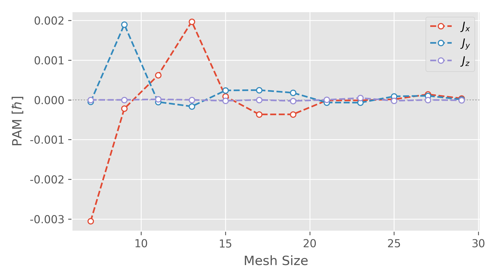
• Convergence test of total PAM with respect to different q-grid sizes

  • First, generate phonon mesh data with different mesh sizes.

    1 2 3 4 5 6 7

    ATOM_NAME = Zn O DIM = 2 2 2 MESH = 29 29 29 # Change the mesh size here GAMMA_CENTER = .TRUE. EIGENVECTORS = .TRUE. MESH_SYMMETRY = .FALSE. # Turn-off symmetry! MESH_FORMAT = HDF5 # use hdf5 format to reduce file size

  • Second, calculate the grid-dependent total PAM

    1 2 3 4 5 6 7 8 9 10 11 12 13

    import h5py import numpy as np for ii in range(7, 30, 2): ph_mesh = h5py.File('mesh_{}.hdf5'.format(ii), 'r') freq = np.array(ph_mesh['frequency']) nqpts, nbnds = freq.shape pvec = np.array(ph_mesh['eigenvector']).reshape((nqpts, nbnds, -1, 3)) natoms = pvec.shape[2] pham = phonon_angular_momentum(freq, pvec) total_pham = (1. / nqpts) * np.sum(pham, axis=(1,2)) print(f'{ii:2d}', total_pham[0], total_pham[1], total_pham[2])

  

  As can be clearly seen, the total PAM for ZnO, when converged, is INDEED ZERO.

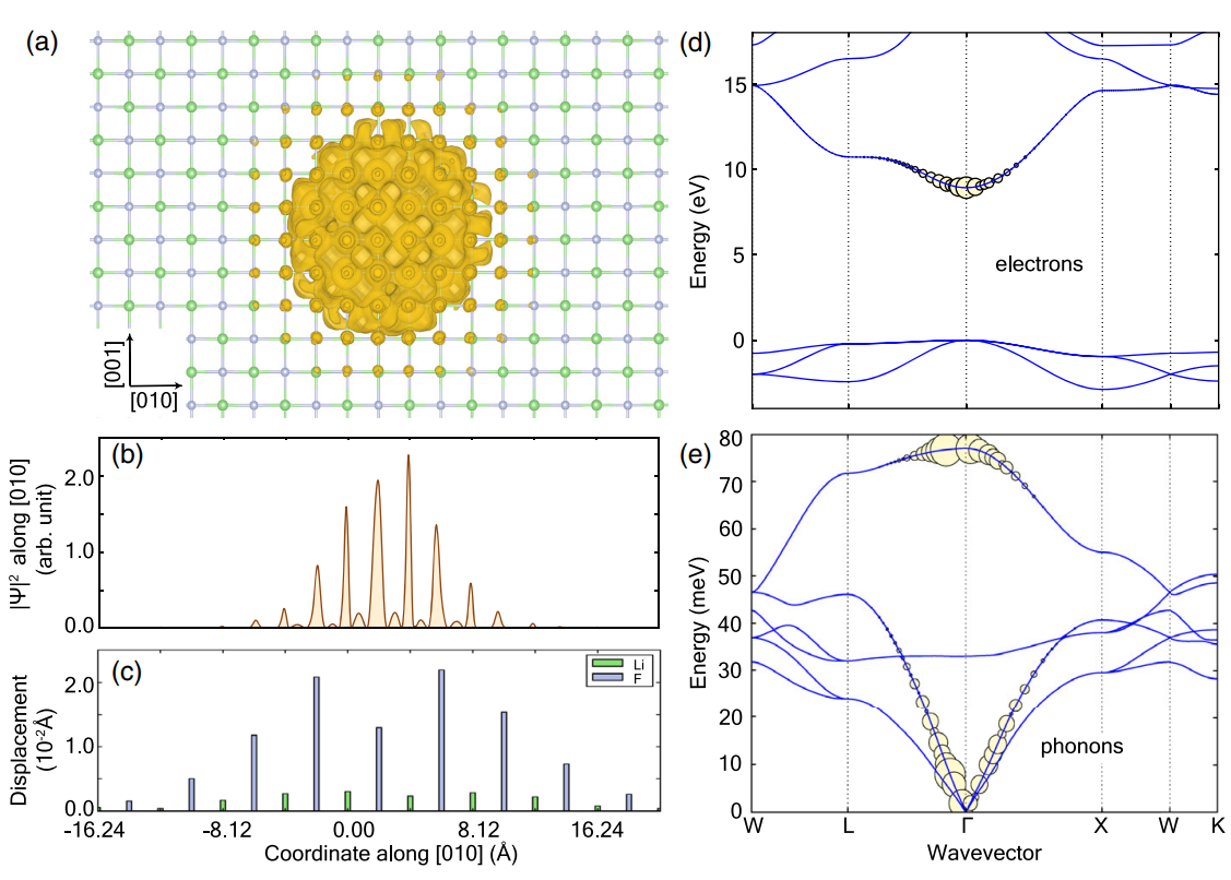
Change of Angular Momentum in Polaron Formation

A polaron is a quasiparticle in which the extra charged carrier is surrounded by cloud of phonons. ⁸ Wio et al. showed that the electronic component of the polaron can be expressed as a coherent superposition of the unperturbed Kohn-Sham wavefunction and the lattice distortion can be expanded by a linear combination of phonon eigenmodes. ⁹

where $P$ is the index of the unit cell, $\kappa$ is the index of the atom within the unit cell and $N_P$ is the number of unit cells.

$|B_{\mathbf{q}\nu}|^2$ can be interpreted as the number of phonons taking part in the polaron formation. In other words, the polaron formation brings the phonon system off-equilibrium, on top of the thermal Bose distribution, and therefore the change of the phonon angular momentum during the polaron formation can be written as

In order to get $B_{\mathbf{q}\nu}$, one can perform the inverse Fourier transform on Eq.\eqref{eq:polaron_ph_part}, by multiplying the left-hand side with $ \boldsymbol\epsilon^{\kappa}_{\mathbf{q}’\nu’} \, e^{-i\mathbf{q}’ \cdot \mathbf{R}_P} $, and then summing over $P$ and $\kappa$. Additionally, one must take into account of the following relations: ¹⁰

Consequently, one gets the following expression for $B_{\mathbf{q}\nu}^*$.

That is, one first performs Fourier transform on $\Delta \boldsymbol \tau_\kappa^P$, then projects the results onto the polarization vectors.

Recall that the phonon frequencies and polarization vectors follow these relations: ¹⁰

Substituting Eq.\eqref{eq:ph_freq_vec_sym} into Eq.\eqref{eq:Bqv}, one has ¹¹

One can then conclude, combining Eq.\eqref{eq:Bqv_sym}, Eq.\eqref{eq:pam_change_in_polaron_formation} and Eq.\eqref{eq:zero_pam_sym}, that the total phonon angular momentum change during the polaron formation is ZERO.

Orbital Angular Momentum

The orbital angular momentum (OAM) for a finite non-interacting system is defined as

For an infinite periodic crystal, the wavefunctions $\psi_n$ are replaced by the Bloch states $\psi_{n\mathbf{k}}$, i.e.

Apparently, the position operator $\mathbf{r}$ is well-defined for finite system, and therefore the OAM for finite system is computable no matter how large the system is. However, the problem arises when we are considering the OAM of crystal, in which case the position measured from some origin increases linearly with distance while the system repeat itself from unit cell to unit cell, and as a result the position operator is ill-defined. The problem is similar to the case of calculating the electric polarization in crystal, where the position operator is also ill-defined and was solved by reformulating the problem in the Wannier representation. ¹²

Modern theory of orbital magnetization (the orbital magnetization is related to the orbital angular momentum) that allows for a rigorous calculation of the magnetic of periodic cyrstals has also been developed in the last decade. ¹³

There are two contributions to the OAM: one from the local atomic OAM and the other emerging from the itinerant motion of the electrons on the surface of the material. Surprisingly, the latter contribution is expressible entirely in terms of bulk quantities. ¹⁴

Atomic-center Approximation

Traditionally, the common approach to avoid the difficulty with the position operator is to use the physically motivated assumption that the OAM is an atomic property, i.e. the OAM mainly originates from the regions near the atom cores. The approach neglects the contribution from the itinerant motion of the electrons and is often referred to as the atomic-center approximation or the muffin-tin approximation.

Within the PAW sphere, the Bloch states can be expressed as

where $\tilde p_j$ and $\phi_j$ are the projector function and the AE partial waves, respectively. ¹⁵ Consequently, the OAM under the atomic-center approximation reads

For the evaluation of inner product of the projector function and PSWFC, please refer the previous post. ¹⁵ Let us now focus on the matrix element of the angular momentum operator between the all-electron partial waves. As has been said, ¹⁵ the AE partial waves can be written as mutiplication of radial and angular parts, i.e.

Therefore, the matrix elements of the angular momentum operator between the Ae partial waves are given by

Note that real spherical harmonics $Z_{lm}$ are used in Eq.\eqref{eq:ae_pwfc}, which are themselves not eigenfunctions of the momentum operator $\hat{L}_z$ and $\mathbf{L}^2$. Instead, the eigenfunctions of $\hat{L}_z$ and $\mathbf{L}^2$ are the complex spherical harmonics $Y_{lm}$, i.e.

The x/y components of the angular momentum operator $\hat{L}_x$/$\hat{L}_y$ are related to the ladder operator $\hat{L}_\pm$ by

And the application of the ladder operators on the spherical harmonics give

As a result, the matrix elements of the angular momentum operators between the complex spherical harmonics can be given

To get the matrix elements of $\mathbf{L}$ between real spherical harmonics, reamember that $Z_{lm}$ and $Y_{lm}$ can be inter-transformed by a unitary matrix $U^l$,¹⁶ i.e.

As a result, one gets

Or in matrix form

1
2
3
4
5
6
7
8
9
10
11
12
13
14
15
16
17
18
19
20
21
22
23
24
25
26
27
28
29
30
31
32
33
34
35
36
37
38
39
40
41
42
43
44
45
46
47
48
49
50
51
52
53
54
55
56

#!/usr/bin/env python
# -*- coding: utf-8 -*-

import numpy as np

def oam_mat_elem(l: int=1, lreal=True):
    '''
    Matrix elements of angular momentum operator between the real/complex
    spherical harmonics.
    '''

    TLP1     = 2*l + 1
    sqrt2inv = 1.0 / np.sqrt(2.0)

    U  = np.zeros((TLP1, TLP1), dtype=complex)
    Lc = np.zeros((3, TLP1, TLP1), dtype=complex)

    for ii in range(TLP1):
        m = ii - l

        # the complex 2 real unitary matrix
        if (m < 0):
            U[ii, ii] = 1j * sqrt2inv
            U[ii, -(ii+1)] = -1j * (-1)**m * sqrt2inv
        if (m == 0):
            U[ii, ii] = 1.0
        if (m > 0):
            U[ii, -(ii+1)] = sqrt2inv
            U[ii, ii] = (-1)**m * sqrt2inv

        # matrix elements of L between complex spherical harmonics
        C_UP = np.sqrt((l-m) * (l+m+1)) / 2
        C_DW = np.sqrt((l+m) * (l-m+1)) / 2
        # fill L_x
        if ((m+1) <= l):
            Lc[0, ii+1, ii] = C_UP
        if ((m-1) >= -l):
            Lc[0, ii-1, ii] = C_DW
        # fill L_y
        if ((m+1) <= l):
            Lc[1, ii+1, ii] = -1j * C_UP
        if ((m-1) >= -l):
            Lc[1, ii-1, ii] =  1j * C_DW
        # fill L_z
        Lc[2, ii, ii] = m

    Lr = U.conj() @ (Lc @ U.T)

    if lreal:
        return Lr
    else:
        return Lc
    

if __name__ == "__main__":
    print(oam_mat_elem(l=1))

Reference