Introduction
Let’s consider an ionic crystal with atomics charges $q_\alpha$ at $\boldsymbol\tau_\alpha$ and $\sum q_\alpha = 0$, where $\alpha$ runs from 1 to the number of atoms in a unit cell. For each unit cell, the Coulomb contribution to the potential energy is then given by
\[\begin{equation} U^{t} = \frac{1}{2} \sum_\alpha q_\alpha \cdot \varphi_{[\alpha]} = \frac{1}{2} \sum_\alpha \sum_\beta \sideset{}{'}\sum_L q_\alpha q_\beta \frac{1}{ | \boldsymbol{\tau}_\beta - \boldsymbol{\tau}_\alpha + \mathbf{R}_L | } \label{eq:ewaldsum_tot} \end{equation}\]-
$\varphi_{[\alpha]}$ is the electrostatic potential at the position of ion $\alpha$, i.e. $\boldsymbol\tau_\alpha$, which is generated by all the other ions except $\alpha$.
\[\begin{equation} \varphi_{[\alpha]}= \sum_\beta \sideset{}{'}\sum_L q_\beta \frac{1}{ | \boldsymbol{\tau}_\beta - \boldsymbol{\tau}_\alpha + \mathbf{R}_L | } \end{equation}\]The prime in the above sum and Eq.\eqref{eq:ewaldsum_tot} means that when $L=0$, $\beta \ne \alpha$.
-
$\boldsymbol\tau_\beta$ and $\mathbf{R}_L$ are the position vector of the $\beta$-th atom in a unit cell and the lattice vector of the $L$-th unit cell, respectively.
-
The summation in Eq.\eqref{eq:ewaldsum_tot} is a conditionally convergent series, which means that the summation is only convergent with some particular summation order if it ever converges.
Ewald Summation
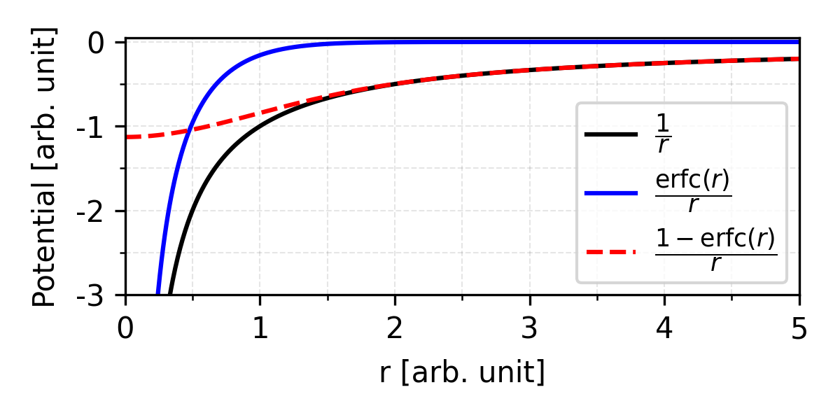
The basic idea of Ewald summation is to introduce a fast decay function $f(\lambda r)$ and rewrite the long-range Coulomb interaction as a sum of two terms:
\[\begin{equation} \frac{1}{r} = {\color{blue}\frac{f(\lambda r)}{r}} + {\color{red}\frac{1 - f(\lambda r)}{r}} \label{eq:coulomb_pot_sep} \end{equation}\]where $\lambda$ is the parameter that determines how fast the function decays.
-
The short-range term can be summed in real-space. The quicker $f(\lambda r)$ decays, the faster the sum converges.
-
The slow-decaying term, however, is short-range in reciprocal-space and thus should be summed in reciprocal space.
-
In Ewald summation, complementary error function is chosen as the decay function. 1
\[\begin{equation} \operatorname{erfc}(r) = 1- \operatorname{erf}(r) \qquad \operatorname{erf}(r) = \frac{2}{\sqrt\pi} \int_0^r e^{-t^2} \,\mathrm{d}t; \end{equation}\]
Physically, the separation of the long-range interaction in Eq.\eqref{eq:coulomb_pot_sep} is realized by first augmenting the point charges at each site with a smooth-varying charge distribution of opposite sign, which effectively screens the point charge and makes the interaction short-range. Subsequently, another smooth-varying charge distribution of the same shape but with same sign as the point charges is introduced.2 The electrostatic potential at position $\boldsymbol\tau_\alpha$ can then be written as linear combination of two terms
\[\begin{equation} \varphi_{[\alpha]} = \varphi_{[\alpha]}^a + \varphi_{[\alpha]}^b \end{equation}\]
If we chosed complementary error function as the decay function in Eq.\eqref{eq:coulomb_pot_sep}, then the smooth-varying compensation charge is of the shape of a Gaussian distribution, i.e.
\[\begin{equation} \rho_\beta^g(\mathbf{r} - \mathbf{r}_0) = -q_\beta (\lambda^2 / \pi)^\frac{3}{2} \exp(-\lambda^2 |\mathbf{r} - \mathbf{r}_0|^2) \label{eq:comp_gaussian_charge} \end{equation}\]where the broadening parameter is $1/\sqrt{2}\lambda$.
Real-space summation
Let’s first inspect the electrostatic potential generated by charge distribution (a). Seen from a greater distance, a Gaussian charge cloud resembles a delta-like point charge, effectively compensating the original charge it accompanies. The effect of distribution (a) is therefore best computed in real-space, where the series will converge quite rapidly. The convergence will be faster if the Gaussians are narrow, i.e. if the parameter $\lambda$ in \eqref{eq:comp_gaussian_charge} is large.
The potential at $\boldsymbol\tau_\alpha$ in the first unit cell generated by another point charge $\beta$ located at the L-th unit cell,
\[\begin{equation} \varphi_1 = \frac{q_\beta}{ |\boldsymbol\tau_\beta + \mathrm{R}_L - \boldsymbol\tau_\alpha| } \end{equation}\]As proved in the appendix, the potential generated by the Gaussian compensation charge can be written as
\[\begin{equation} \varphi_2 = -q_\beta \frac{\operatorname{erf}{ \lambda |\boldsymbol\tau_\beta + \mathrm{R}_L - \boldsymbol\tau_\alpha| }}{ |\boldsymbol\tau_\beta + \mathrm{R}_L - \boldsymbol\tau_\alpha| } \end{equation}\]Summing over $\beta$ and $L$, one have
\[\begin{equation} U^{r} = \frac{1}{2} \sum_\alpha q_\alpha \cdot \varphi_{[\alpha]}^a = \frac{1}{2} \sum_\alpha \sum_\beta \sideset{}{'}\sum_L q_\alpha q_\beta \frac{\operatorname{erfc}{(\lambda | \boldsymbol{\tau}_\beta - \boldsymbol{\tau}_\alpha + \mathbf{R}_L | )}}{ | \boldsymbol{\tau}_\beta - \boldsymbol{\tau}_\alpha + \mathbf{R}_L | } \label{eq:ewaldsum_real} \end{equation}\]Reciprocal-space summation
Now let’s focus on the electrostatic potential generated by smooth charge distribution (b).
\[\begin{equation} \rho^b(\mathbf{r}) = \sum_L \sum_\beta -q_\beta \rho^g(\mathbf{r} - \boldsymbol\tau_\beta - \mathbf{R}_L) \end{equation}\]By performing Fourier transform and utlizing the shifting property of FT, one have
\[\begin{equation} \tilde\rho^b(\mathbf{k}) = \frac{1}{\sqrt{N\Omega}} \sum_\beta \sum_L -q_\beta \tilde\rho^g_0(\mathbf{k}) e^{-\mathbf{k}\cdot\boldsymbol\tau_\beta} e^{-\mathbf{k}\cdot\mathbf{R}_L} \label{eq:rho_b_ft_k} \end{equation}\]Where $N$ and $\Omega$ are the number and volume of unit cells, respectively.
\[\begin{equation} \tilde\rho^g_0(\mathbf{k}) = (\lambda^2/\pi)^{\frac{3}{2}} \int \exp(-\lambda^2 r^2) \,\mathrm{d}\mathbf{r} = e^{-k^2/4\lambda^2} \end{equation}\]Remember that
\[\begin{equation} \sum_L e^{-\mathbf{k}\cdot\mathbf{R}_L} = N \,\delta_{\mathbf{k}, \mathbf{G}} \end{equation}\]i.e. the Fourier component is only non-zero if $\mathbf{k}$ equals the reciprocal lattice vectors $\mathbf{G}$. As a result, Eq.\eqref{eq:rho_b_ft_k} reduces to
\[\begin{equation} \tilde\rho^b(\mathbf{G}) = \sqrt{\frac{N}{\Omega}} \sum_\beta -q_\beta\, e^{-G^2/4\lambda^2} e^{-\mathbf{G}\cdot\boldsymbol\tau_\beta} \label{eq:rho_b_ft_G} \end{equation}\]The charge and electrostatic potential are related by Poisson’s equation
\[\begin{equation} -G^2\, \tilde\varphi^g(\mathbf{G}) = 4\pi\tilde\rho^g(\mathbf{G}) \end{equation}\]By performing inverse Fourier transform, one have
\[\begin{align} \varphi^b(\mathbf{r}) &= \frac{1}{\sqrt{N\Omega}} \sum_{\mathbf{G}} -\frac{4\pi\tilde\rho^b(\mathbf{G})}{G^2} \, e^{i\mathbf{G}\cdot\mathbf{r}} \nonumber \\ &= \frac{1}{\Omega} \sum_{\mathbf{G}} \sum_\beta q_\beta \frac{4\pi}{G^2} \, e^{-G^2/4\lambda^2} \, e^{i\mathbf{G}\cdot(\mathbf{r} - \boldsymbol\tau_\beta)} \end{align}\]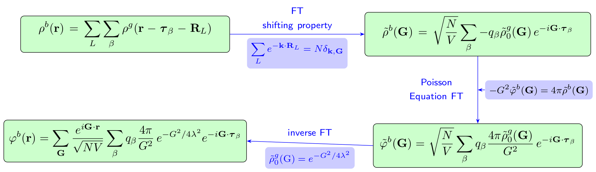
As a result, the contribution of charge distribution to the potential energy writes
\[\begin{equation} U^{g} = \frac{1}{2} \sum_\alpha q_\alpha \cdot \varphi_{[\alpha]}^b(\boldsymbol\tau_\alpha) = \frac{1}{2 V} \sum_\alpha \sum_\beta \sum_\mathbf{G\ne0} q_\alpha q_\beta \frac{4\pi}{G^2} \, e^{-G^2/4\lambda^2} e^{-i\mathbf{G}\cdot(\boldsymbol\tau_\alpha - \boldsymbol\tau_\beta)} \label{eq:ewaldsum_recp} \end{equation}\]Self-interaction term
In Eq.\eqref{eq:ewaldsum_recp}, one has included a spurious term that originates from the interaction of point charge $q_\alpha$ and the Gaussian charge distribution, which should be removed. As proved in the appendix, the electrostatic potential at the center of the Gaussian charge distribution is $q_\alpha\frac{2\lambda}{\sqrt\pi}$, therefore this self-interaction term can be written as
\[\begin{equation} U^s = \frac{1}{2}\sum_\alpha q_\alpha^2 \frac{2\lambda}{\sqrt\pi} \end{equation}\]
Total Ewald sum
Energy
The total potential energy can then be written
\[\begin{align} \label{eq:ewaldsum_all_eq} U^{t} &= U^{r} +U^{g} -U^{s} \\[6pt] U^{r} & = \frac{1}{2} \sum_\alpha \sum_\beta \sideset{}{'}\sum_L q_\alpha q_\beta \frac{\operatorname{erfc}{(\lambda | \boldsymbol{\tau}_\beta - \boldsymbol{\tau}_\alpha + \mathbf{R}_L | )}}{ | \boldsymbol{\tau}_\beta - \boldsymbol{\tau}_\alpha + \mathbf{R}_L | } \\[6pt] U^{g} &= \frac{1}{2 V} \sum_\alpha \sum_\beta \sum_\mathbf{G\ne0} q_\alpha q_\beta \frac{4\pi}{G^2} \, e^{-G^2/4\lambda^2} e^{-i\mathbf{G}\cdot(\boldsymbol\tau_\alpha - \boldsymbol\tau_\beta)} \\[6pt] U^{s} &= \sum_\alpha {q_\alpha^2} \frac{\lambda}{\sqrt{\pi}} \end{align}\]Forces
In molecular dynamics, one often requies the evaluation of forces on atoms. By simply differentiating the energy over position $\boldsymbol\tau$, one can get the expression for forces.
\[\begin{align} F^t_{\alpha,p} &= F^r_{\alpha,p} + F^g_{\alpha,p},\qquad\qquad (p=x,y,z) \\[9pt] F^r_{\alpha,p} &= -\frac{\partial U^r}{\partial \tau_{\alpha,p}} = q_\alpha \sum_{\beta\ne\alpha} \sum_L q_\beta \frac{(R_{\alpha\beta,L})_p}{R^3_{\alpha\beta,L}} \left[ \operatorname{erfc}(\lambda R_{\alpha\beta,L}) + \frac{2\lambda}{\sqrt\pi} R_{\alpha\beta,L} e^{-\lambda^2R_{\alpha\beta,L}^2} \right], \\[6pt] F^g_{\alpha,p} &= -\frac{\partial U^g}{\partial \tau_{\alpha,p}} = \frac{4\pi}{V} \sum_{\beta\ne\alpha} \sum_\mathbf{G\ne0} q_\alpha q_\beta \frac{G_p}{G^2} \, e^{-G^2/4\lambda^2} \sin\left[ \mathbf{G}\cdot(\boldsymbol\tau_\beta - \boldsymbol\tau_\alpha) \right] \end{align}\]where we have defined
\[\begin{equation} R_{\alpha\beta,L} = | \boldsymbol{\tau}_\beta - \boldsymbol{\tau}_\alpha + \mathbf{R}_L | \end{equation}\]Examples: Madelung constants
The Ewald summation has been implemented in python in the VaspBandunfolding package. Below we will use the Ewald summation to evaluate the Madelung constant, one can find the relating files in VaspBandunfolding/examples/ewald
1
2
3
4
5
6
7
8
9
10
11
12
13
14
15
16
17
18
19
20
21
22
23
24
25
26
27
28
29
30
31
32
33
34
35
36
37
38
39
40
41
#!/usr/bin/env python

import numpy as np
from ase.io import read
from ewald import ewaldsum

if __name__ == '__main__':

    crystals = [
        'NaCl.vasp',
        'CsCl.vasp',
        'ZnO-Hex.vasp',
        'ZnO-Cub.vasp',
        'TiO2.vasp',
        'CaF2.vasp',
    ]

    ZZ = {
        'Na':  1, 'Ca':  2,
        'Cl': -1,  'F': -1,
        'Cs':  1,
        'Ti':  4,
        'Zn':  2,
         'O': -2,
    }

    print('-' * 41)
    print(f'{"Crystal":>9s} | Ref Atom | {"Madelung Constant":>18s}')
    print('-' * 41)

    for crys in crystals:
        atoms = read(crys)
        esum = ewaldsum(atoms, ZZ)

        # print(esum.get_ewaldsum())
        M = esum.get_madelung()
        C = crys.replace('.vasp', '')
        R = atoms.get_chemical_symbols()[0]
        print(f'{C:>9s} | {R:^8s} | {M:18.12f}')

    print('-' * 41)
the output
1
2
3
4
5
6
7
8
9
10
-----------------------------------------
  Crystal | Ref Atom |  Madelung Constant
-----------------------------------------
     NaCl |    Na    |     1.747564594633
     CsCl |    Cs    |     1.762674773071
  ZnO-Hex |    Zn    |     1.640553196154
  ZnO-Cub |    Zn    |     1.638055053389
     TiO2 |    Ti    |     3.018317142868
     CaF2 |    Ca    |     3.276110106778
-----------------------------------------
Appendix
Fourier transform of Gaussian
For a 1D Gaussian $g(x) = e^{-\alpha x^2}$, the Fourier transform is given by
\[\begin{align} {\cal F}[g](k) & = \int\limits_{-\infty}^\infty e^{-\alpha x^2} e^{-ikx} \,\mathrm{d}x = e^{-k^2/4\alpha}\int\limits_{-\infty}^\infty e^{-\alpha (x+\frac{ik}{2\alpha})^2} \,\mathrm{d}x \nonumber\\ & = \sqrt{\frac{\pi}{\alpha}} e^{-k^2/4\alpha} \qquad\Leftarrow\qquad \int\limits_{-\infty}^\infty e^{-a (z+b)^2} \,\mathrm{d}z = \sqrt{\frac{\pi}{a}} \end{align}\]Note that we have omitted the normlization factor $(q/2\pi)^{D/2}$ in the above Fourier transform.
-
Apparently, the Fourier transform of 1D Gaussian is also a Gaussian, except that it is in the reciprocal space and the broadening parameter changes from $q/\sqrt{2\alpha}$ to $\sqrt{2\alpha}$.
-
The conclusion applies to 2D and 3D Gaussian:
\[\begin{align} g(x,y) = e^{-\alpha(x^2 + y^2)} \quad&\Rightarrow\quad {\cal F}[g](k_x, k_y) % = % \int_{-\infty}^\infty % e^{-\alpha(x^2 + y^2)} % e^{-ik_x x -ik_y y} % \, \mathrm{d}x \mathrm{d}y = \frac{\pi}{a} e^{-(k_x^2 + k_y^2)/4\alpha} \\ g(x,y,z) = e^{-\alpha(x^2 + y^2 + z^2)} \quad&\Rightarrow\quad {\cal F}[g](k_x, k_y, k_z) = \left(\frac{\pi}{a}\right)^{\frac{3}{2}} e^{-(k_x^2 + k_y^2 + k_z^2)/4\alpha} \end{align}\]
Electrostatic potential of Gaussian charge distribution
For a given charge distribution,
\[\rho^g(r) = q\, (\lambda^2 / \pi)^\frac{3}{2} \exp(-\lambda^2 r^2)\]the electrostatic potential is determined by the Poisson equation, i.e.
\[\begin{equation} \nabla^2 \varphi^g(\mathbf{r}) = 4\pi \rho^g(\mathbf{r}) \end{equation}\]or in reciprocal space
\[\begin{equation} -G^2\, \tilde\varphi^g(\mathbf{G}) = 4\pi\tilde\rho^g(\mathbf{G}) \label{eq:poisson_ft} \end{equation}\]As has been proved in previous section, we have
\[\begin{equation} \tilde\rho^g(\mathbf{G}) = \frac{q}{(2\pi)^{\frac{3}{2}}}\,e^{-G^2/4\lambda^2} \label{eq:ft_gaussian_charge} \end{equation}\]Substituting Eq.\eqref{eq:ft_gaussian_charge} into Eq.\eqref{eq:poisson_ft}, we have
\[\begin{equation} \tilde\varphi^g(\mathbf{G}) = -q \frac{4\pi}{G^2} e^{-G^2/4\lambda^2} \label{eq:elecpot_ft} \end{equation}\]By performing inverse Fourier transform on Eq.\eqref{eq:elecpot_ft}, one can have
\[\begin{align} \varphi^g(\mathbf{r}) &= \frac{1}{(2\pi)^{\frac{3}{2}}}\int\, \tilde\varphi^g(\mathbf{G})\, e^{i\mathbf{G}\cdot\mathbf{r}} \,\mathrm{d}\mathbf{r} = - \frac{q}{8\pi^3}\int\, \frac{4\pi}{G^2} e^{-G^2/4\lambda^2}\, e^{i\mathbf{G}\cdot\mathbf{r}} \,\mathrm{d}\mathbf{r} \nonumber \\ &= -\frac{q}{2\pi^2} \int_0^\infty \int_0^\pi \frac{1}{G^2} e^{-G^2/4\lambda^2}\, e^{iGr\cos\theta} 2\pi G^2\sin\theta \,\mathrm{d}G\,\mathrm{d}\theta \nonumber\\ &= \frac{q}{\pi r} \int_0^\infty e^{-G^2/4\lambda^2} \frac{1}{iG} \left[ e^{iGr} - e^{-iGr} \right] \,\mathrm{d}G \nonumber \\ &= \frac{q}{\pi r} {\color{red}\int\limits_{-\infty}^\infty e^{-G^2/4\lambda^2} \frac{1}{iG} \, e^{iGr} \,\mathrm{d}G} \label{eq:elecpot_ift} \end{align}\]Now, define the red term in the above equation as $I(r)$. Obviously, we can have the following relation
\[\begin{align} \frac{\mathrm{d}I(r)}{\mathrm{d} r} &= \int\limits_{-\infty}^\infty e^{-G^2/4\lambda^2}\, e^{iGr} \,\mathrm{d}G = \left(4\pi\lambda^2\right)^{\frac{1}{2}} e^{-\lambda^2 r^2}\\ \Rightarrow \quad I(r) &= \left(4\pi\lambda^2\right)^{\frac{1}{2}} \int_0^r e^{-\lambda^2 \tau^2} \,\mathrm{d}\tau = \pi \operatorname{erf}{(\lambda r)} \end{align}\]By putting the expression of $I(r)$ back to Eq.\eqref{eq:elecpot_ft}, we can have
\[\begin{equation} \varphi^g(\mathbf{r}) = = \frac{q}{r} \frac{2}{\sqrt\pi} \int_0^{\lambda r} e^{-\tau^2}\, \mathrm{d}\tau = q \frac{\operatorname{erf}(\lambda r)}{r} \end{equation}\]-
For $r\to 0$, we can assume that $e^{-\tau^2} \approx 1$ and $\operatorname{erf}(\lambda r) \approx \lambda r$, as a result
\[\begin{equation} \varphi^g(r=0) = q\frac{2\lambda}{\sqrt{\pi}} \end{equation}\]
Reference
-
Daan Frenkel and Berend Smit, Understanding Molecular Simulation: From Algorithms to Applications ↩