Introduction
Let’s start with a parametric 1D Hamiltonian $H(r)$
\[\begin{equation} H(r) = \begin{pmatrix} \varepsilon_1^d(r) & \lambda(r) \\[6pt] \lambda(r) & \varepsilon_2^d(r) \end{pmatrix} \end{equation}\]where the dependence of the the matrix elements on the parameter $r$ are assumed to be
\[\begin{align} \varepsilon_1^d(r) &= \phantom{-}\alpha\cdot r \\[6pt] \varepsilon_2^d(r) &= -\alpha\cdot r \\[6pt] \lambda(r) &= \gamma \cdot e^{-r^2 / \beta^2} \end{align}\]Obviously, the derivative of the Hamiltonian with respect to $r$ can be written as
\[\begin{equation} \nabla_r H(r) = \begin{pmatrix} \alpha & -\frac{2\gamma}{\beta^2}\cdot r \cdot e^{-r^2/\beta^2} \\[6pt] -\frac{2\gamma}{\beta^2}\cdot r\cdot e^{-r^2/\beta^2} & -\alpha \end{pmatrix} \end{equation}\]The eigenvalues of the Hamiltonian can be solved analytically,
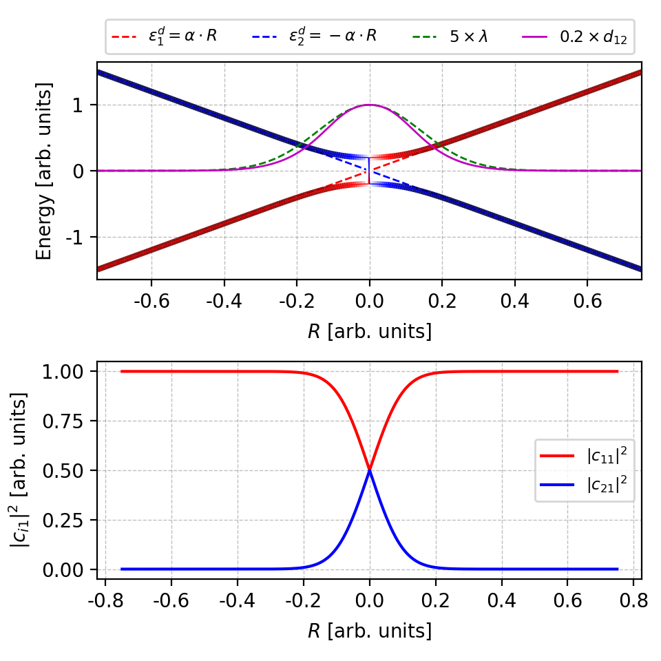
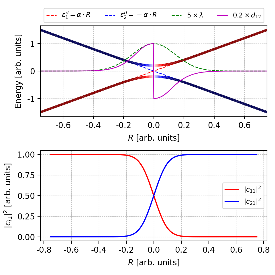
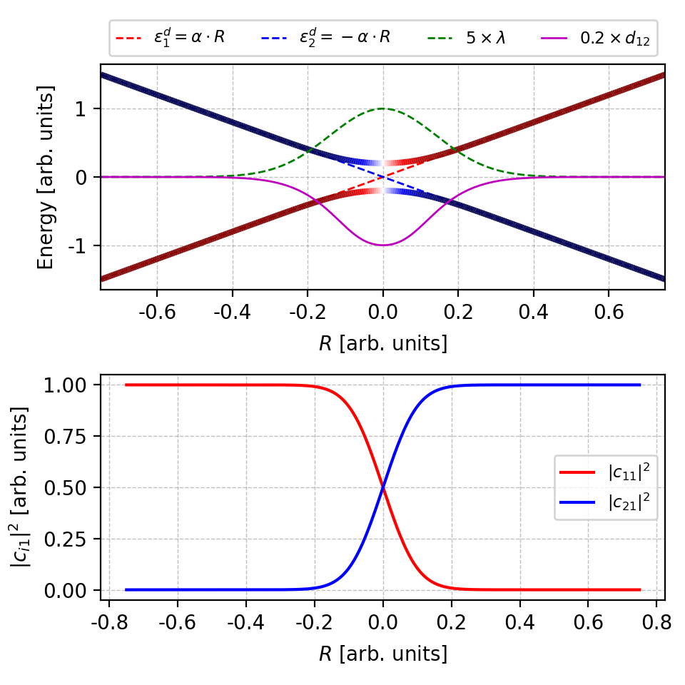
\[\begin{align} \varepsilon_i^a &= \frac{(\varepsilon_1^d + \varepsilon_2^d)}{2} \pm \frac{ \sqrt{(\varepsilon_1^d - \varepsilon_2^d)^2 + 4\lambda^2} }{2} \\[6pt] &= \pm \sqrt{\alpha^2\cdot r^2 + \gamma^2\cdot e^{-2r^2/\beta^2}} \qquad (i=1,2) \label{eq:eig_val} \end{align}\]Apparently, the energy gap at $r=0$ is $\Delta \varepsilon = 2\lambda$.
The corresponding eigenvectors can also be obtained
\[\begin{align} \psi_i^a &= \begin{pmatrix} \dfrac{-2\lambda}{ (\varepsilon_1^d - \varepsilon_2^d) \mp \sqrt{(\varepsilon_1^d - \varepsilon_2^d)^2 + 4\lambda^2} } \\[12pt] 1 \end{pmatrix} \\[12pt] &= \begin{pmatrix} \dfrac{-\gamma\cdot e^{-r^2/\beta^2}}{ \alpha r \mp \sqrt{\alpha^2\cdot r^2 + \gamma^2\cdot e^{-2r^2/\beta^2}} } \\[12pt] 1 \end{pmatrix} \label{eq:eig_vec} \end{align}\]Note that the above eigenvectors is NOT normalized and should therefore be properly normalized when implemented in codes.
1
2
3
4
5
6
7
8
9
10
11
12
13
14
15
#!/usr/bin/env python

import sympy as sp
from sympy.matrices import Matrix

E1, E2, L = sp.symbols("E1 E2 L")
Hamil = Matrix([
    [E1, L],
    [L, E2],
])

sp.pprint(Hamil.eigenvects())

# U, T = Hamil.diagonalize(normalize=True)
# sp.pprint(U)
The nonadiabatic coupling vector (NAC), which is a scalar in 1D, can now be written as
\[\begin{align} d_{ij} &= \frac{ \langle \psi_i |\nabla_r H(r)|\psi_j \rangle }{ \varepsilon_j^a -\varepsilon_i^a } \\[9pt] & = \dfrac{ \begin{pmatrix} c_{i1}^* & c_{i2}^* \end{pmatrix} \cdot \begin{pmatrix} \alpha & -\frac{2\gamma}{\beta^2}\cdot r \cdot e^{-r^2/\beta^2} \\[6pt] -\frac{2\gamma}{\beta^2}\cdot r\cdot e^{-r^2/\beta^2} & -\alpha \end{pmatrix} \cdot \begin{pmatrix} c_{j1} \\[6pt] c_{j2} \end{pmatrix} }{ (\varepsilon_j^a - \varepsilon_i^a) } \end{align}\]In practice, the derivative of the Hamiltonian with respect to $r$ is hard to get and we often evaluate another quantity $D_{ij} = d_{ij}\cdot\dot{r}$, which is also referred to as nonadiabatic coupling.
\[\begin{align} D_{ij} & = \frac{ \langle \psi_i |\nabla_r H(r)|\psi_j \rangle }{ \varepsilon_j^a -\varepsilon_i^a }\cdot\dot r = \langle \psi_i | \frac{\partial}{\partial t} | \psi_j \rangle \\[9pt] &\approx \dfrac{ \langle \psi_i(t) |\psi_j(t+\Delta t)\rangle - \langle \psi_i(t+\Delta t) |\psi_j(t)\rangle }{ 2\Delta t } \end{align}\]where the finite difference approximation in the second line was proposed by Hammes-Schiffer and Tully (HST).1
Below, we show an example results of the model Hamiltonian:
1
2
3
4
5
6
7
8
9
10
11
12
13
14
15
16
17
18
19
20
21
22
23
24
25
26
27
28
29
30
31
32
33
34
35
36
37
38
39
40
41
42
43
44
45
46
47
48
49
50
51
52
#!/usr/bin/env python

import numpy as np

rmax = 0.75
nr   = 501
rr   = np.linspace(-rmax, rmax, nr, endpoint=True)

alpha = 2.0; beta  = 0.20; gamma = 0.20

E1 = alpha * rr
E2 = -alpha * rr
W0 = gamma * np.exp(-rr**2 / beta**2)

# The Hamiltonian
Ham = np.zeros((nr, 2, 2))
Ham[:,0,0] = E1
Ham[:,1,1] = E2
Ham[:,0,1] = W0
Ham[:,1,0] = W0

# The derivative of Hamiltonian to R
Hderv = np.zeros((nr, 2, 2))
Hderv[:,0,0] = alpha
Hderv[:,1,1] = -alpha
Hderv[:,0,1] = -2 * rr * W0 / beta**2
Hderv[:,1,0] = -2 * rr * W0 / beta**2

E3 = -np.sqrt(alpha**2 * rr**2 + W0**2)
E4 = -E3

V3 = np.array([
    -W0 / (alpha*rr + np.sqrt(alpha**2 * rr**2 + W0**2)),
    np.ones(nr)
]).T
# normalization
V3 /= np.linalg.norm(V3, axis=1)[:,None]
V4 = np.array([
    -W0 / (alpha*rr - np.sqrt(alpha**2 * rr**2 + W0**2)),
    np.ones(nr)
]).T
# normalization
V4 /= np.linalg.norm(V4, axis=1)[:,None]

nac = np.sum(
    V3 * np.matmul(Hderv, V4[...,None])[:,:,0], axis=1
) / (E4 - E3)

# |c_11|^2
rho_1 = V3[:,0]**2
# |c_21|^2
rho_2 = V4[:,0]**2

-
Let us now focus on the NAC at $r = 0$, where
\[\begin{equation} \psi_1 = \begin{pmatrix} \frac{1}{\sqrt{2}} \\[6pt] \frac{1}{\sqrt{2}} \end{pmatrix}; \qquad \psi_2 = \begin{pmatrix} \frac{-1}{\sqrt{2}} \\[6pt] \frac{1}{\sqrt{2}} \end{pmatrix}; \qquad \nabla_r H(r) = \begin{pmatrix} \alpha & 0 \\[6pt] 0 & -\alpha \end{pmatrix} \end{equation}\]One can show that at $r = 0$,
\[\begin{equation} d_{12}(r=0) = \frac{\alpha}{(\varepsilon_1^a - \varepsilon_2^a)} = \frac{\alpha}{2\lambda} \end{equation}\]i.e. the NAC is inversely propotional to the energy gap at $r = 0$, which is consistent with the adiabatic theorem.2
One should not confuse the external perturbation $\lambda$ with NAC.
-
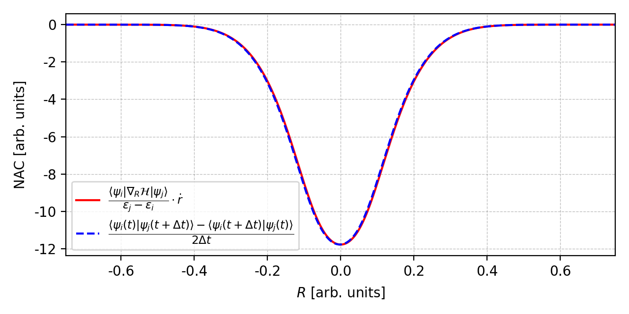
Comparison of $D_{ij}$ from two methods. Suppose that the parameter $r$ follows the motion of a harmonic oscillator, i.e.
\[\begin{align} r &= -r_0 \cdot\cos(\omega t) \\[6pt] \dot r &= \omega\,r_0\cdot\sin(\omega t) \end{align}\]
Figure 2. Comparison of the nonadiabatic coupling from two different methods. The figure is plotted by this script.
Band Ordering and Phase Correction
When the eigenvalues and eigenvectors are obtained numerically, there can be problems with the ordering of the band (eigenvalues may not be properly ordered) and the phase of the wavefunction (arbitrary phase can be assigned to the eigenvectors), both of which may affect the calculation of the NAC.
-
No band reordering and NO phase correction.
1
2
3
4
vals, vecs = np.linalg.eig(Ham)
E3, E4 = vals.T
V3 = vecs[...,0]
V4 = vecs[...,1]
Eigenvalues returned by
numpy.linalg.eigare not necessarily ordered, usenumpy.linalg.eighinstead, which arrange the eigenvalues in ascending order. Here, we usenumpy.linalg.eigonly to show the effects of band ordering.
Figure 3. One can clearly see a band crossing near $r=0$ in the upper panel, whereas in the lower panel the coefficients $|c|^2$ are not smooth (a kink) at the same place. However, the NAC only differ by a sign factor to the correct NAC. The figure is plotted by this script. What if we introduce more artificial band crossings?
1
2
3
4
5
6
7
8
9
10
11
12
# use np.linalg.eigh to get the correct band order and then reshuffle it
vals, vecs = np.linalg.eigh(Ham)

# randomize the band order
oo = np.random.randint(2, size=(nr))
xx = oo - 1

E3 = vals[range(nr),oo]
E4 = vals[range(nr),xx]

V3 = vecs[range(nr),:,oo]
V4 = vecs[range(nr),:,xx]
Figure 4. The energies, NACs and coefficients $|c_{i1}|^2$ with more artificial band crossings. The figure is plotted by this script. -
With more artificial band crossings, as shown in the upper left panel, the wavefunction coefficients $|c_{i1}|^2$ in the upper right panel shows many abrupt changes. However, the overall envelope shape is correct.
-
The NACs in the lower panel also become unsmooth with many abrupt changes. Moreover, there are envelopes enclosing the NAC curve. The lower and upper envelope are the correct NAC and that differ by a sign factor, respectively.
-
-
With band reordering and NO phase correction.
1
2
3
4
5
6
7
8
9
10
11
12
13
14
vals, vecs = np.linalg.eig(Ham)
E3, E4 = vals.T
V3 = vecs[...,0]
V4 = vecs[...,1]

oo = np.asarray(E3 <= E4, dtype=int)
xx = oo - 1
# band reorder --- energy
E3 = vals[range(nr),xx]
E4 = vals[range(nr),oo]

# band reorder --- wavefunction
V3 = vecs[range(nr),:,xx]
V4 = vecs[range(nr),:,oo]
Figure 5. With band re-ordering, the artificial band crossing is now gone and the coefficients are correct, too. Howover, the NAC change signs near $r=0$. The figure is plotted by this script. -
With band reordering and With phase correction.
1
2
3
4
5
6
7
8
9
10
11
12
13
14
15
16
17
18
vals, vecs = np.linalg.eig(Ham)
E3, E4 = vals.T
V3 = vecs[...,0]
V4 = vecs[...,1]

oo = np.asarray(E3 <= E4, dtype=int)
xx = oo - 1
# band reorder --- energy
E3 = vals[range(nr),xx]
E4 = vals[range(nr),oo]

# band reorder --- wavefunction
V3 = vecs[range(nr),:,xx]
V4 = vecs[range(nr),:,oo]

# phase correction
V3[V3[:,1] < 0] *= -1
V4[V4[:,1] < 0] *= -1
Figure 6. With band re-ordering and phase correction, the results are in consistent with Fig.1 The figure is generated by this script. Reference