
Introduction
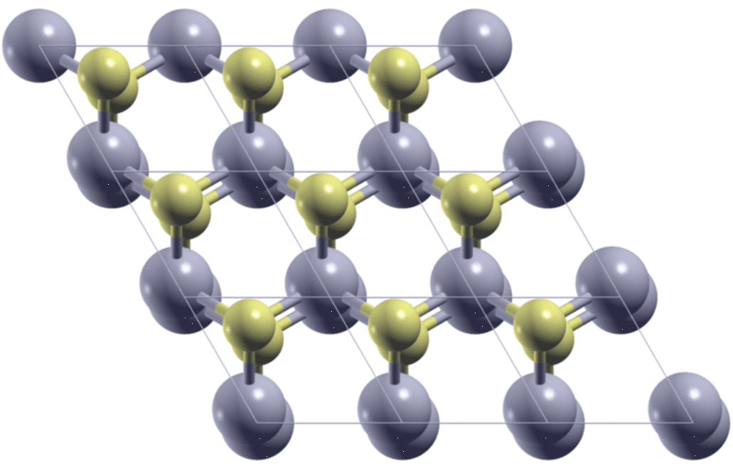
A few days ago, I met a problem so that I needed to calculate the stacking-dependent energy of bilayer MoS2. As is shown in the figure below, by shifting one of the two layers relative to the other, I got many different structures. I need to know what are the energies of these structures.
Structure generation
The first step is to generate the structures. Here, starting from the AA
stacking of the bilayer MoS2, I move the top layer in the x/y
direction with a step of $\frac{1}{9}\vec{a} + \frac{1}{9}\vec{b}$, i.e. 10
points in each direction, where $\vec{a}$ and $\vec{b}$ are the basis vectors of
the 2D cell. The upper and lower layers are shifted by a vector
-
Note that the number of points is chosen to be $3n + 1$ so that the special stackings with shifting vectors $\frac{1}{3}\vec{a} + \frac{2}{3}\vec{b}$ and $\frac{2}{3}\vec{a} + \frac{1}{3}\vec{b}$ are both sampled.
-
Due the periodic boundary condition (PBC) $l/k = 1$ is the same as $l/k = 0$, therefore we removed those structures in the script. However, we will need to consider the PBC lateron in the data processing.
1
2
3
4
5
6
7
8
9
10
11
12
13
14
15
16
17
18
19
20
21
22
23
24
25
26
27
28
29
30
31
32
33
34
35
36
37
38
39
40
41
42
43
44
45
46
#!/usr/bin/env python
# -*- coding: utf-8 -*-

import os
import numpy as np
from ase.io import read, write
from ase.constraints import FixScaled

# load the starting geometry
geo0 = read('p0.vasp')
pc0  = geo0.get_scaled_positions().copy()

# only allow movement in z-direction
cc = []
for ii in range(len(geo0)):
    cc.append(FixScaled(geo0.cell, ii, [1, 1, 0]))
geo0.set_constraint(cc)

# number of points in x/y direction
nx = ny = 10

# Due to PBC, remove the other borders [:,:-1, :-1]
dxy = np.mgrid[0:1:1j*nx, 0:1:1j*ny][:,:-1,:-1].reshape((2,-1)).T
nxy = np.mgrid[0:nx, 0:ny][:,:-1,:-1].reshape((2,-1)).T

# the indeices of the atoms in the upper/lower layer
L1   = [ii for ii in range(len(geo0)) if pc0[ii,-1] < 0.5]
L2   = [ii for ii in range(len(geo0)) if pc0[ii,-1] >= 0.5]
assert len(L1) + len(L2) == len(geo0)

for ii in range(nxy.shape[0]):
    dx, dy = dxy[ii]
    ix, iy = nxy[ii]

    pc = pc0.copy()
    # only move the atoms in the upper layer
    pc[L2] += [dx, dy, 0]
    geo0.set_scaled_positions(pc)

    # python 3
    # os.makedirs('{:02d}-{:02d}'.format(ix, iy), exist_ok=True)
    # python 2
    if not os.path.isdir('{:02d}-{:02d}'.format(ix, iy)):
        os.makedirs('{:02d}-{:02d}'.format(ix, iy))

    write("{:02d}-{:02d}/POSCAR".format(ix, iy), geo0, direct=True, vasp5=True)
After execution of the script, there shoule be 81 directories in the current
working directory, each with a POSCAR in it.
1
2
3
4
5
6
7
8
# ls
00-00  00-07  01-05  02-03  03-01  03-08  04-06  05-04  06-02  07-00  07-07  08-05
00-01  00-08  01-06  02-04  03-02  04-00  04-07  05-05  06-03  07-01  07-08  08-06
00-02  01-00  01-07  02-05  03-03  04-01  04-08  05-06  06-04  07-02  08-00  08-07
00-03  01-01  01-08  02-06  03-04  04-02  05-00  05-07  06-05  07-03  08-01  08-08
00-04  01-02  02-00  02-07  03-05  04-03  05-01  05-08  06-06  07-04  08-02
00-05  01-03  02-01  02-08  03-06  04-04  05-02  06-00  06-07  07-05  08-03
00-06  01-04  02-02  03-00  03-07  04-05  05-03  06-01  06-08  07-06  08-04
The two numbers in the name of the directories represent the $l$ and $k$ of the shifting vector.
Geometry optimization
The next step is to perform geometry optimization run within each directory.
To do that, prepare INCAR, KPOINTS, POTCAR and VASP submission file in
the current directory and them create symbolic links in each sub-directory.
1
2
3
4
5
6
7
8
9
10
11
for ii in ??-??/
do
    cd ${ii}

    ln -sf ../INCAR
    ln -sf ../KPOINTS
    ln -sf ../POTCAR
    ln -sf ../sub_vasp

    cd ../
done
Submit the jobs and wait until all the VASP jobs are finished. You may want to
check that all the jobs are indeed converged. This can be done with the
following line of command.
1
ls ??-??/OUTCAR | xargs -I {} bash -c '(grep "reached require" {} >& /dev/null || echo {})'
If all the jobs are fully converged, the output of the last line should be
empty. Otherwise, enter the output directories, move CONTCAR to POSCAR and
resubmit the job.
Postprocessing
At this step, we first read the total energies of each structure
1
2
3
4
5
6
7
8
9
10
11
12
13
14
15
16
17
18
19
20
21
22
23
24
25
#!/usr/bin/env python
# -*- coding: utf-8 -*-

import os
import numpy as np
from ase.io import read

# number of points in x/y direction
nx = ny = 10

if not os.path.isfile('pes_xy.npy'):
    pes = np.zeros((nx-1, ny-1))
    for ii in range(nx-1):
        for jj in range(ny-1):
            pes[ii, jj] = read('{:02d}-{:02d}/OUTCAR'.format(ii, jj)).get_potential_energy()
    np.save('pes_xy.npy', pes)

pes = np.load('pes_xy.npy')
# Apply PBC
pes = np.pad(pes, (0, 1), 'wrap')

# set the minimum to zero
pes -= pes.min()
# eV to meV
pes *= 1000
Remember that we removed the structure with $l/k = 1$, therefore we apply PBC and pad those data with $l/k = 0$.
1
2
# Apply PBC
pes = np.pad(pes, (0, 1), 'wrap')
And finally we are in a position to plot the results.
1
2
3
4
5
6
7
8
9
10
11
12
13
14
15
16
17
18
19
20
21
22
23
24
25
26
27
28
29
30
31
32
33
34
35
36
37
38
39
40
import matplotlib.pyplot as plt
from mpl_toolkits.axes_grid1 import make_axes_locatable

# The 2D cell
cell = [[ 3.190316, 0.000000],
        [-1.595158, 2.762894]]

# the Cartesian coordinates of the shifting vectors
rx, ry = np.tensordot(cell, np.mgrid[0:1:1j*nx, 0:1:1j*ny], axes=(0, 0))

fig = plt.figure(
    figsize=(4.8, 6.0),
    dpi=300
)
axes = [plt.subplot(211), plt.subplot(212)]

for ii in range(2):
    ax = axes[ii]

    ax.set_aspect('equal')

    if ii == 0:
        img = ax.pcolormesh(rx, ry, pes)
    else:
        img = ax.contourf(rx, ry, pes)

    ax.set_xlabel(r'$x$ [$\AA$]', labelpad=5)
    ax.set_ylabel(r'$y$ [$\AA$]', labelpad=5)

    divider = make_axes_locatable(ax)
    ax_cbar = divider.append_axes('right', size=0.15, pad=0.10)
    plt.colorbar(img, ax_cbar)

    ax_cbar.text(0.0, 1.05, 'meV',
                 ha='left',
                 va='bottom',
                 transform=ax_cbar.transAxes)

plt.tight_layout(pad=1)
plt.show()
The output
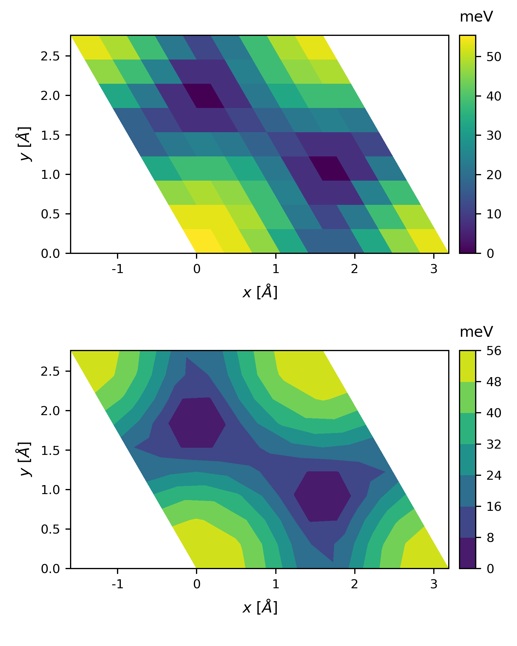
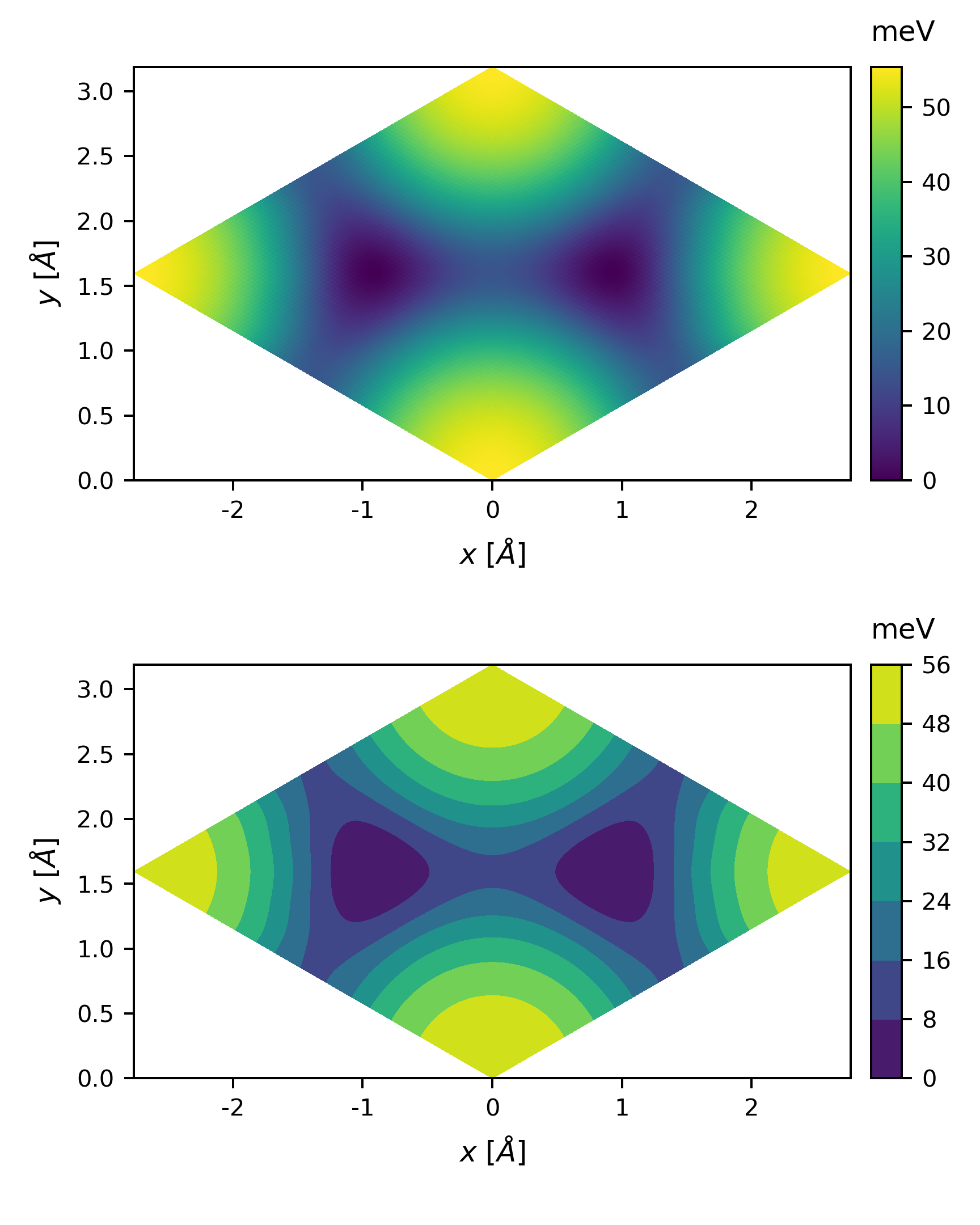
By changing the basis vectors to
1
2
cell = [[ 2.762894, 1.595158],
        [-2.762894, 1.595158]]
we get

The plot looks a little coarse, we can perform a 2D interpolation before plotting
1
2
3
4
5
6
7
8
9
10
11
12
13
# 2D interpolation
from scipy.interpolate import interp2d

N      = 100
x0     = np.linspace(0, 1, nx)
y0     = np.linspace(0, 1, ny)
x1     = np.linspace(0, 1, N)
y1     = np.linspace(0, 1, N)

fpes   = interp2d(x0, y0, pes, kind='cubic')
PES    = fpes(x1, y1)

Rx, Ry = np.tensordot(cell, np.mgrid[0:1:1j*N, 0:1:1j*N], axes=(0, 0))
and in the plotting part
1
2
3
4
if ii == 0:
    img = ax.pcolormesh(Rx, Ry, PES)
else:
    img = ax.contourf(Rx, Ry, PES)
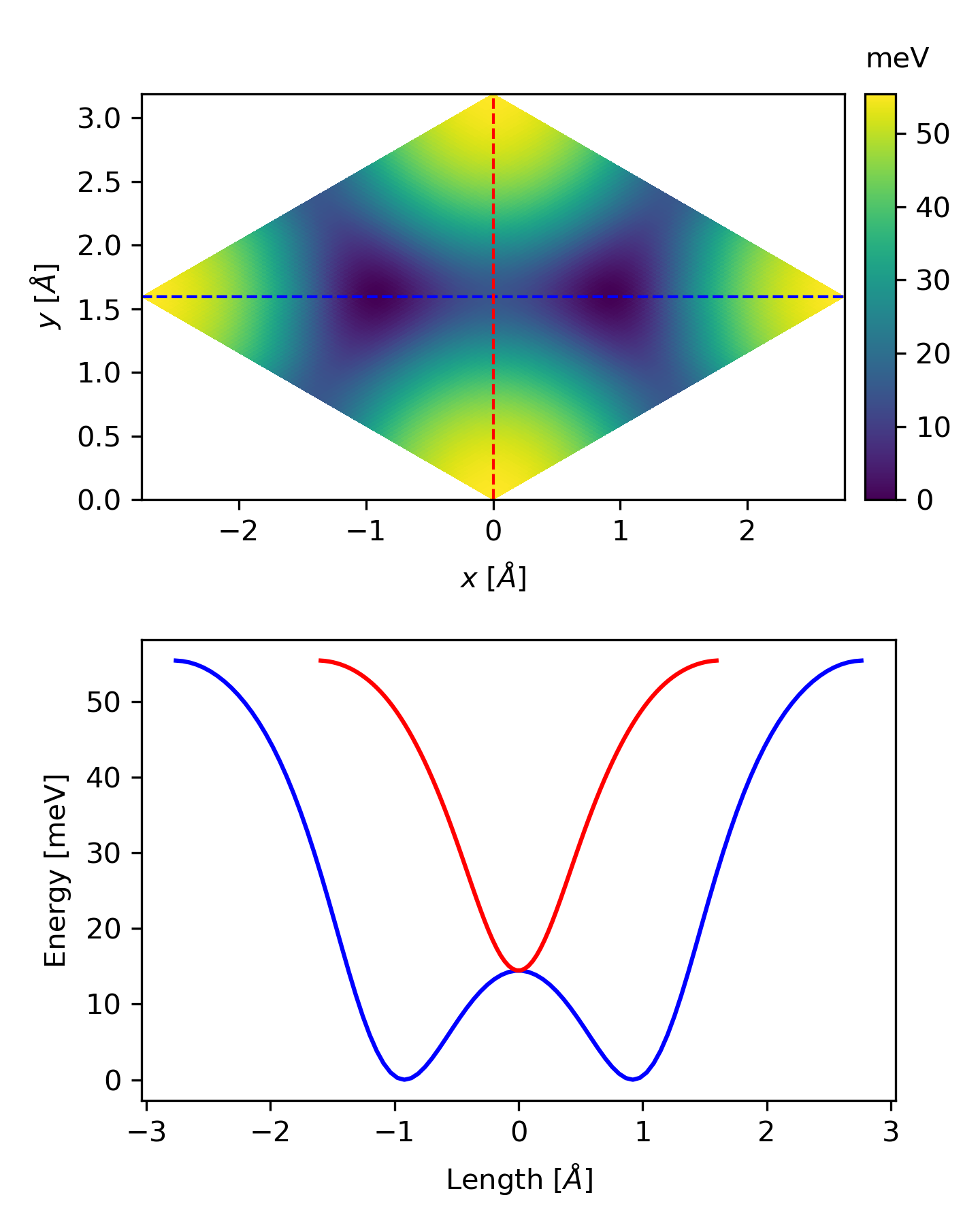
Sometimes, the colormap might not be so intuitive, we can also plot the potential energy along some direction. All we need is a little modification of the above code.
1
2
3
4
5
6
7
8
9
10
11
12
13
14
15
16
17
18
19
20
21
22
23
24
25
26
27
28
29
30
31
32
33
34
35
36
37
38
39
40
41
42
43
44
45
46
47
48
49
50
51
52
53
54
55
56
57
58
59
idx = range(N)
############################################################
fig = plt.figure(
    figsize=(4.8, 6.0),
    dpi=300
)
axes = [plt.subplot(211), plt.subplot(212)]

for ii in range(2):
    ax = axes[ii]

    if ii == 0:
        ax.set_aspect('equal')
        img = ax.pcolormesh(Rx, Ry, PES)

        ax.plot(Rx[idx, idx[::-1]], Ry[idx, idx[::-1]],
                ls='--', lw=1.0, color='b')
        ax.plot(Rx[idx, idx], Ry[idx, idx],
                ls='--', lw=1.0, color='r')

        divider = make_axes_locatable(ax)
        ax_cbar = divider.append_axes('right', size=0.15, pad=0.10)
        plt.colorbar(img, ax_cbar)

        ax_cbar.text(0.0, 1.05, 'meV',
                     ha='left',
                     va='bottom',
                     transform=ax_cbar.transAxes)

        ax.set_xlabel(r'$x$ [$\AA$]', labelpad=5)
        ax.set_ylabel(r'$y$ [$\AA$]', labelpad=5)
    else:
        L1 = np.r_[
            [0],
            np.cumsum(
                np.linalg.norm(
                    np.diff(
                        np.array([Rx[idx, idx[::-1]], Ry[idx, idx[::-1]]]),
                        axis=1
                    ),
                    axis=0)
            )
        ]
        L2 = np.r_[
            [0],
            np.cumsum(
                np.linalg.norm(
                    np.diff(
                        np.array([Rx[idx, idx], Ry[idx, idx]]),
                        axis=1
                    ),
                    axis=0)
            )
        ]
        ax.plot(L1 - L1.max() / 2, PES[idx, idx[::-1]], color='b')
        ax.plot(L2 - L2.max() / 2, PES[idx, idx], color='r')

        ax.set_xlabel(r'Length [$\AA$]', labelpad=5)
        ax.set_ylabel(r'Energy [meV]', labelpad=5)
The related files can be downloaded here.