Origin of High Harmonic Peak in Fourier Transform of Time-dependent Kohn-Sham Energies

Introduction

When performing ab initio molecular dynamics, one often can obtain the time evolution of Kohn-Sham energies $\epsilon_n(t)$, as is shown schematically in the figure below.

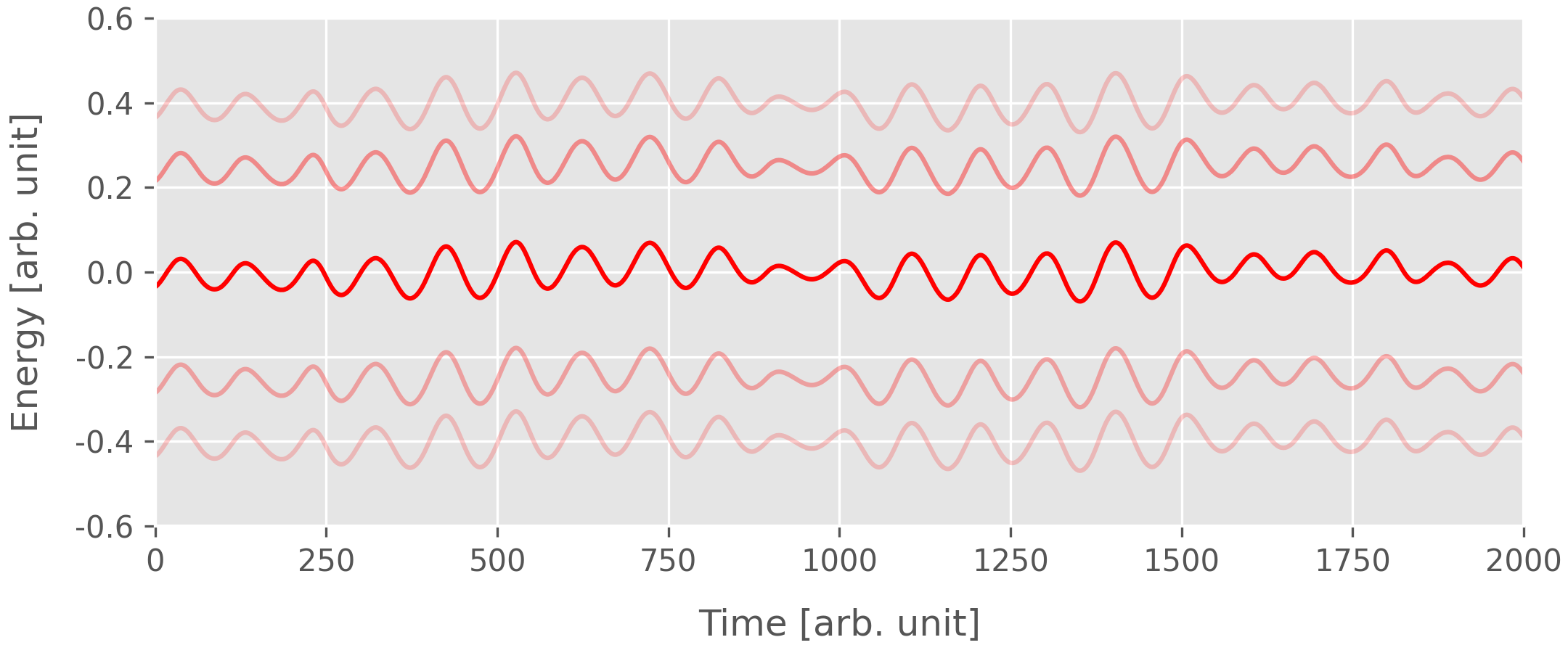
By performing Fourier transform on $\epsilon_n(t)$, one can have information as to which of the phonon modes couples to the selected Kohn-Sham state by, for example, comparing the peaks in the Fourier spectra with Raman experiments or first-principles results. However, one often can also find peaks in the Fourier spectra at frequency $\omega$ well beyond the maximum frequency of all the phonon modes $\omega_{\text{max}}$, i.e. $\omega > \omega_{\text{max}}$, the so-called higher harmonics. This can be understood by time-independent perturbation theory.

A simple explanation

As is well-known, within the DFT Kohn-Sham formalism, the Kohn-Sham energies $\epsilon_n$ are eigenvalues of the following equation:

where the effective Kohn-Sham potential $ V_{\text{KS}}(\mathbf{r}; \lbrace\mathbf{R}\rbrace)$ depends implicitly on the nuclear coordinates. By expanding the Kohn-Sham effective potential in terms of the nuclear displacement $u^P_{\kappa\alpha}$ from their equilibrium positions $\lbrace\mathbf{R}_0 \rbrace$, the potential to second order in the displacements can be written as

where the indices $P/L$ run over the unit cells, $\kappa$ over the atom within the cell and $\alpha/\beta$ stand for $x/y/z$ components of the displacements.

The Kohn-Sham Hamiltonian can then be separated into two parts:

where

By treating $\mathcal{H}_{\text{ep}}$ term as perturbation and using the time-independent perturbation theory,¹ one can have the correction to the Kohn-Sham energies

where $\epsilon_n^0$ and $\psi_n(\mathbf{r})$ are eigenenergies and eigenfunctions of $\mathcal{H}_0$. The two terms on the right-hand-side of Eq.\eqref{eq:energy_first_order} comes from the first-order correction of $\mathcal{H}_{\text{ep}}$, and the term in Eq.\eqref{eq:energy_second_order} derives from the second-order correction of the linear term in Eq.\eqref{eq:H_epc}.

• In the simplest case, when there is only one atom that is displaced from equilibrium by an amount $u$, then one can drop the summation and write the energy correction as

  \[\begin{align} \Delta\epsilon_n &= \langle{\psi^0_n}|{\frac{\partial V_{\text{KS}}}{\partial R^P_{\kappa\alpha}}}|{\psi^0_n}\rangle \,\textcolor{red}{u} + \frac{1}{2} \langle{\psi^0_n}|{\frac{\partial^2 V_{\text{KS}}}{\partial^2 R^P_{\kappa\alpha}}}|{\psi^0_n}\rangle \textcolor{red}{u^2} + \sum_{m\ne n} \frac{ \left|\langle{\psi^0_m}|{\displaystyle\frac{\partial V_{\text{KS}}}{\partial R^P_{\kappa\alpha}}}|{\psi^0_n}\rangle\right|^2 }{\epsilon_n^0 - \epsilon_m^0} \textcolor{red}{u^2} \\[3pt] &\equiv A_1\cdot u + A_2\cdot u^2 \end{align}\]

  where we have denote the coefficients of the linear and quadratic terms as $A_1$ and $A_2$, respectively. Now, if the atom further oscillate with a frequency $\omega_0$, i.e. $u(t) \varpropto cos(\omega_0 t)$, then there will be peaks at $\omega_0$ and $2\omega_0$ in the Fourier transform of $\Delta\epsilon_n(t)$ due to the quadratic term.

• More generally, one can write the nuclear displacements as superposition of normal modes,² i.e.

  \[\begin{equation} u_{\kappa\alpha}^P = \frac{2}{\sqrt{N_P}} \sum_{\mathbf{q}} \sum_{\nu} l_{\mathbf{q}\nu} \, \chi_{\mathbf{q}\nu}^{\kappa\alpha} Q_{\mathbf{q}\nu}^* \, e^{i\mathbf{q}\cdot\mathbf{R}_P} \label{eq:disp_normal_modes} \end{equation}\]

  where $l_{\mathbf{q}\nu}$ is the “zero-point” displacement amplitude of the $\nu$-th phonon mode with momentum $\mathbf{q}$:

  \[\begin{equation} l_{\mathbf{q}\nu} = \sqrt{\frac{\hbar}{2M_{\kappa}\omega_{\mathbf{q}\nu}}} \end{equation}\]

  $\chi_{\mathbf{q}\nu}^{\kappa\alpha}$ is the corresponding phonon polarization vector.

  Substituting Eq.\eqref{eq:disp_normal_modes} into Eq.\eqref{eq:energy_first_order} and Eq.\eqref{eq:energy_second_order}, one can have

  \[\begin{align} \Delta\epsilon_n &= \frac{2}{\sqrt{N_P}} \sum_{\mathbf{q}\nu} Q_{\mathbf{q}\nu}^* \sum_{P\kappa\alpha} \textcolor{red}{ \langle{\psi^0_n}|{\frac{\partial V_{\text{KS}}}{\partial R^P_{\kappa\alpha}}}|{\psi^0_n}\rangle } \, l_{\mathbf{q}\nu} \, \chi_{\mathbf{q}\nu}^{\kappa\alpha} \, e^{i\mathbf{q}\cdot\mathbf{R}_P} \label{eq:1st_correction_normal_modes} \\[6pt] &\quad+ \sum_{\mathbf{q}\nu} \sum_{\mathbf{q}'\nu'} Q_{\mathbf{q}\nu}^* Q_{\mathbf{q}'\nu'}^* \times \frac{1}{2} \sum_{P\kappa\alpha} \sum_{L\lambda\beta} \langle{\psi^0_n}|{\frac{\partial^2 V_{\text{KS}}}{\partial R^P_{\kappa\alpha}\partial R^L_{\lambda\beta}}}|{\psi^0_n}\rangle \frac{4}{N_P} [ l_{\mathbf{q}\nu} \chi_{\mathbf{q}\nu}^{\kappa\alpha} e^{i\mathbf{q}\cdot\mathbf{R}_P} ][ l_{\mathbf{q}'\nu'} \chi_{\mathbf{q}'\nu'}^{\lambda\beta} e^{i\mathbf{q}\cdot\mathbf{R}_L} ] \\[3pt] &\quad+ \sum_{P\kappa\alpha} \sum_{m\ne n} \frac{ \left|\langle{\psi^0_m}|{\displaystyle\frac{\partial V_{\text{KS}}}{\partial R^P_{\kappa\alpha}}}|{\psi^0_n}\rangle\right|^2 }{\epsilon_n^0 - \epsilon_m^0} [ \sum_{\mathbf{q}\nu} Q_{\mathbf{q}\nu}^* \frac{2}{\sqrt{N_P}} l_{\mathbf{q}\nu} \chi_{\mathbf{q}\nu}^{\kappa\alpha} e^{i\mathbf{q}\cdot\mathbf{R}_P} ]^2 \\[6pt] \end{align}\]

  Within the harmonic approximation, the normal modes evolve as:

  \[Q_{\mathbf{q}\nu} \varpropto e^{-i\omega_{\mathbf{q}\nu}t}+e^{i\omega_{\mathbf{q}\nu}t}\]

  Apparently, when performing the Fourier transform on $\Delta\epsilon_n(t)$, the quadratic terms of $Q_{\mathbf{q}\nu}$ will not only introduce peaks at $\omega_{\mathbf{q}\nu}$, but also at $\omega_{\mathbf{q}\nu}\pm\omega_{\mathbf{q}’\nu’}$ in the Fourier spectra.

  Let’s now further rewrite the right-hand-side of Eq.\eqref{eq:1st_correction_normal_modes}, following Eq.(32) to Eq.(38) of Ref. ³, as

  \[\begin{align} &\phantom{ {} ={} } \sum_{P\kappa\alpha} \langle{\psi^0_n} | {\frac{\partial V_{\text{KS}}}{\partial R^P_{\kappa\alpha}}} | {\psi^0_n}\rangle l_{\mathbf{q}\nu}\,\chi_{\mathbf{q}\nu}^{\kappa\alpha}\,e^{i\mathbf{q}\cdot\mathbf{R}_P} \\[3pt] &= \langle{\psi^0_n} | l_{\mathbf{q}\nu} \sum_{\kappa\alpha} e^{i\mathbf{q}\cdot\mathbf{r}} \textcolor{blue}{ \left[ \sum_{P} e^{-i\mathbf{q}\cdot(\mathbf{r}-\mathbf{R}_P)} {\frac{\partial V_{\text{KS}}}{\partial R^P_{\kappa\alpha}}} \right] } \chi_{\mathbf{q}\nu}^{\kappa\alpha} | {\psi^0_n}\rangle \\[3pt] &= \langle{\psi^0_n} \bigl| e^{i\mathbf{q}\cdot\mathbf{r}} \cdot \underbrace{ l_{\mathbf{q}\nu} \sum_{\kappa\alpha} \textcolor{blue}{ \bigl[\partial_{\mathbf{q}}^{\kappa\alpha} v_{\text{KS}}\bigr] } \chi_{\mathbf{q}\nu}^{\kappa\alpha} }_{\textcolor{red}{\displaystyle\Delta_{\mathbf{q}\nu}v_{\text{KS}}}} \bigr| {\psi^0_n}\rangle_{\text{crys}} \\ &= \langle{u^0_n} \bigl| e^{i\mathbf{q}\cdot\mathbf{r}} \cdot \textcolor{red}{\displaystyle\Delta_{\mathbf{q}\nu}v_{\text{KS}}} \bigr| {u^0_n}\rangle_{\text{uc}} \\ &= g_{nn\nu}(\mathbf{k}, \mathbf{q})\, \delta_{\mathbf{q}0} \label{eq:1st_couple_to_gamma} \end{align}\]

  where $\mathbf{k}$ is the crystal momentum of the Kohn-Sham state $\psi_n^0(\mathbf{r}) = N_P^{-1/2}\,e^{i\textbf{k}\cdot\textbf{r}}u_n^0(\textbf{r})$ and $g_{nn\nu}(\mathbf{k}, \mathbf{q})$ is the electron-phonon coupling matrix element. The subscript “crys” and “uc” means that the integration is carried out in the whole crystal and the unit cell, respectively.

  One can conclude from Eq.\eqref{eq:1st_couple_to_gamma} that only those phonon modes with $\mathbf{q}=0$ (or effectively those that fold onto $\Gamma$-point if supercell is used) contribute to the first-order energy correction.

Reference