
Introduction
The supercell (SC) method is the ubiquitous approach for the study of solid-state periodic boundary condition systems. In the simplest case, one just construct an SC by repeating the primitive cell (PC) in the periodic direction a number of times without adding any defects, distortion, doping etc. A direct consequence of this procedure manifest itself in the electronic band structure. As can be seen in Figure 1, the number of bands increases in the SC as compared to that of PC. With a larger real-space cell, the reciprocal-space Brillouin Zone (BZ) will become smaller. As a result, the band structure will fold into the small supercell BZ (SBZ).
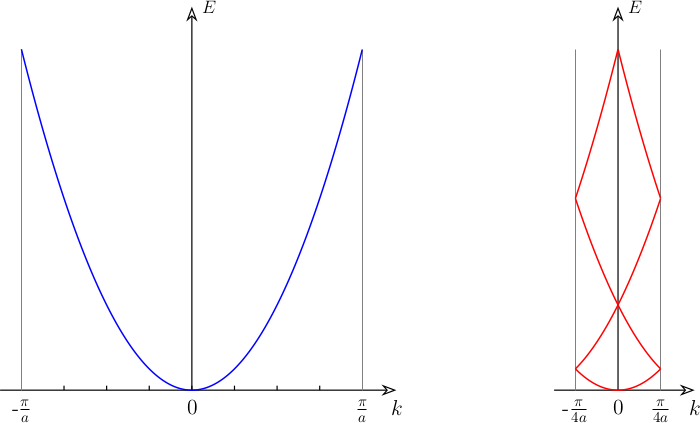
However, supercell calculations are usually performed in order to allow for minor modification of the crystal structure, e.g. defects, distortions etc., to best mimic the real conditions. In this cases it could be useful to investigate, up to what extent, the electronic structure of the original non-defective cell is preserved. To this scope, unfolding the band structure of the SC to the one of the PC becomes handy.
Available codes
There are many codes that can perform the band unfolding procedure.
A bit of notations
Consider the case where the basis vectors of the SC and PC satisfy:
\[ \underline{\vec{A}} = \underline{M}\cdot\underline{\vec{a}} \]
where \(\underline{\vec{A}}\) and \(\underline{\vec{a}}\) are matrices with the cell basis vectors as rows and \(\underline{M}\) the trasformation matrix. As a general convention, capital and lower caseletters indicate quantities in the SC and PC, respectively. A similar relation holds in reciprocal space:
\[ \underline{\vec{B}} = \underline{M}^{-1}\cdot\underline{\vec{b}} \]
1D illustration
Below we will use an 1D example to illustrate the basic idea of band unfoldng. Suppose we have a signal $g_1(t)$ with duration $T$ and time step $\mathrm{d}t$. If we perform Fourier transform (FT) on $g(t)$, i.e. $\mathcal{F}\{g_1\}$, then the maximum frequency in the frequency domain $\Omega_1^{\text{max}}$ is determined by $\mathrm{d}t$ while the frequency spacing is determined by $T$, i.e.
\[\Omega_1^{\text{max}} = {2\pi \over \mathrm{d}t}; \qquad \mathrm{d}\omega_1 = {2\pi \over T}\]Now, if we repeat the signal for another time duration $T$ so that we have a new signal $g_2(t)$ with duration $2T$. When we perform FT, the maximum frequency $\Omega_2^{\text{max}}$ is the same since the time step $\mathrm{d}t$ does not change. However, the frequency spacing $\mathrm{d}\omega_2$ is only half of the original value.
\[\Omega_2^{\text{max}} = {2\pi \over \mathrm{d}t} = \Omega_1^{\text{max}}; \qquad \mathrm{d}\omega_2 = {\pi \over T} = {1\over 2}\mathrm{d}\omega_1\]As a result, these frequencies are shared by both $\mathcal{F}\{g_1\}$ and $\mathcal{F}\{g_2\}$.
\[\omega = 2n\cdot\mathrm{d}\omega_2 = n\cdot\mathrm{d}\omega_1\]Since $g_2(t)$ keeps the original periodicity of $g_1(t)$, the FT should be the same at frequencies $\omega = 2n\cdot\mathrm{d}\omega_2$ or $n\cdot\mathrm{d}\omega_1$.
\[\mathcal{F}\{g_2\}[2n\cdot\mathrm{d}\omega_2] = \mathcal{F}\{g_1\}[n\cdot\mathrm{d}\omega_1]\]Moreover, for those frequencies $\omega = (2n + 1)\cdot\mathrm{d}\omega_2$, the FT should be 0, i.e.
\[\mathcal{F}\{g_2\}[(2n + 1)\cdot\mathrm{d}\omega_2] = 0\]This result can be clearly seen in Figure 2, where we perform FT on one signal with duration $T= 100$ and another signal that is obtained by repeating the original one twice. The FT amplitude at $\omega = 2n\cdot\mathrm{d}\omega_2$ are the same for both signals while the amplitude at $\omega = (2n+1)\cdot\mathrm{d}\omega_2$ for the longer signal is 0. The basic idea of the unfolding is to sum the amplitude at $\omega = 2n\cdot\mathrm{d}\omega_2$,
\[P = \sum_n |\mathcal{F}\{g_2\}[2n\cdot\mathrm{d}\omega_2]|^2\]If the signal is normalized, then $P$ should be 1.
References
- V. Popescu and A. Zunger, “Extracting \(E\) versus \(\vec{k}\) effective band structure from supercell calculations on alloys and impurities”, Phys. Rev. B 85, 085201 (2012)
Band unfolding example
In this section, we will show you how to do band unfolding using
VaspBandUnfolding and
VASP. You will have to first install the VaspBandUnfolding package on your
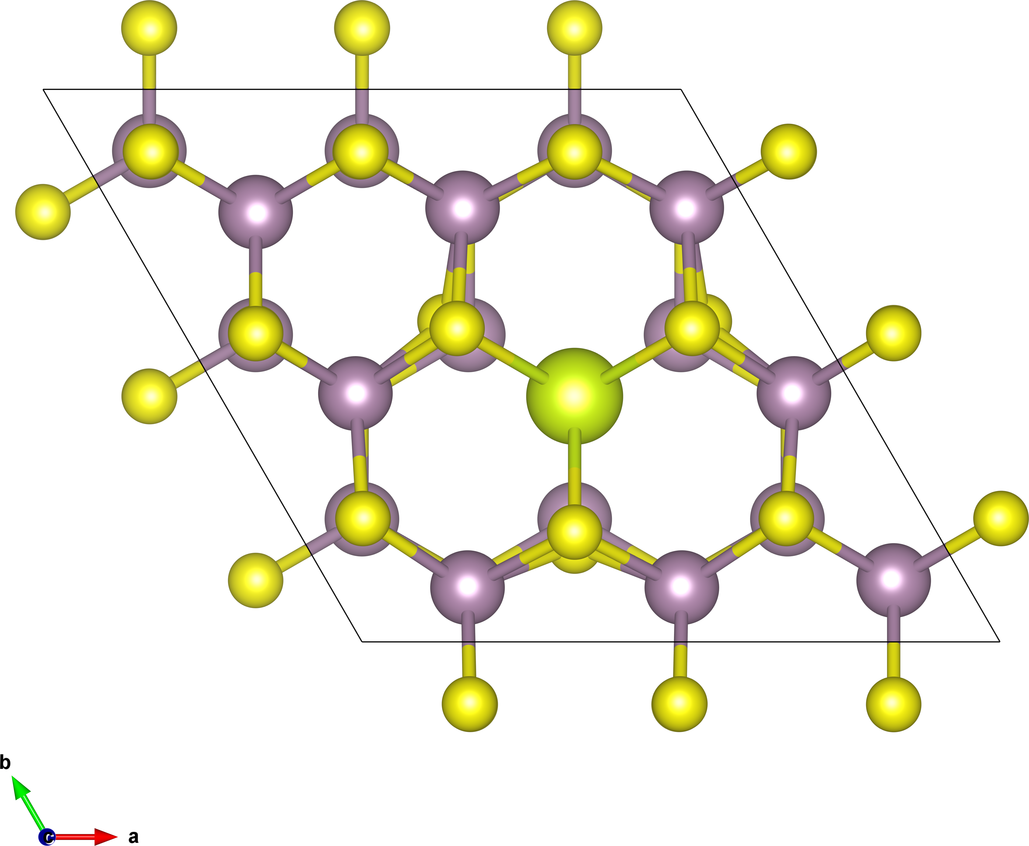
cluster. The system we choose is 3x3x1 Ce-doped bilayer MoS2, as
shown in Figure 3.
For a 3x3x1 SC, the tranformation matrix between SC and PC is
1
2
3
M = [[3.0, 0.0, 0.0],
     [0.0, 3.0, 0.0],
     [0.0, 0.0, 1.0]]
Note, all the calculations that follow are done with the SC.
SCF calculaton
First, perform an SCF calculation with the SC and generate the converged charge
density file CHGCAR. I will not go further into the details of the input files
as any VASP user should be familiar with this step. Special attential should
be paid to the LCHARG tag in INCAR, since will read the CHGCAR file in the
next step.
1
  LCHARG = .TRUE.
NSCF calculaton
In this step, we will read the CHGCAR that we generated in the last step and
perform an NSCF calculation. We will also need to write out the WAVECAR file for
unfolding. For the INCAR file, other than the normal settings, these tags
should be set.
1
2
3
4
  ICHARG = 11
  LCHARG = .FALSE.
  LORBIT = 11
   LWAVE = .TRUE.
In addition, we will need a special KPOINTS file. To do this, first we need to
define the k-point path for the band structure plot. Here, we follow the k-point
path that connect the special high-symmetry points M, G, K and M of the
PC Brillouin Zone. After that, find out the corresponding k-points of the SC on
which those k-points of PC fold. And finally, remove the duplicated ones. Use
the following script to generate the KPOINTS file.
1
2
3
4
5
6
7
8
9
10
11
12
13
14
15
16
17
18
19
20
21
22
23
24
25
26
27
#!/usr/bin/env python
# -*- coding: utf-8 -*-

import os
import numpy as np
from unfold import make_kpath, removeDuplicateKpoints, find_K_from_k, save2VaspKPOINTS

# high-symmetry point of a Hexagonal BZ in fractional coordinate
kpts = [[0.0, 0.5, 0.0],            # M
        [0.0, 0.0, 0.0],            # G
        [1./3, 1./3, 0.0],          # K
        [0.0, 0.5, 0.0]]            # M

# create band path from the high-symmetry points, 30 points inbetween each pair
# of high-symmetry points
kpath = make_kpath(kpts, nseg=30)
K_in_sup = []
for kk in kpath:
    kg, g = find_K_from_k(kk, M)
    K_in_sup.append(kg)

# remove the duplicate K-points
reducedK, kmap = removeDuplicateKpoints(K_in_sup, return_map=True)

if not os.path.isfile('KPOINTS'):
    # save to VASP KPOINTS
    save2VaspKPOINTS(reducedK)
Do NOT forget to copy the CHGCAR in the last step to the current directory.
With all the necessary files, submit the job and run VASP.
Postprocessing
When the NSCF calculation is finished, we can then proceed plot the unfolded
band structure. Make sure that you write out the WAVECAR file.
1
2
3
4
5
6
7
8
9
10
11
12
13
14
15
16
17
18
19
20
21
22
23
24
25
26
27
28
29
30
31
32
33
34
35
36
37
38
39
40
41
42
43
44
45
46
47
48
49
50
51
52
53
54
55
56
57
58
59
60
61
62
63
64
65
66
67
68
69
#!/usr/bin/env python
# -*- coding: utf-8 -*-

import os
import numpy as np
from procar import procar
from unfold import unfold, EBS_scatter
from unfold import make_kpath, removeDuplicateKpoints, find_K_from_k, save2VaspKPOINTS


# The tranformation matrix between supercell and primitive cell.
M = [[3.0, 0.0, 0.0],
     [0.0, 3.0, 0.0],
     [0.0, 0.0, 1.0]]

# high-symmetry point of a Hexagonal BZ in fractional coordinate
kpts = [[0.0, 0.5, 0.0],            # M
        [0.0, 0.0, 0.0],            # G
        [1./3, 1./3, 0.0],          # K
        [0.0, 0.5, 0.0]]            # M

# basis vector of the primitive cell
cell = [[ 3.1903160000000002,    0.0000000000000000,    0.0000000000000000],
        [-1.5951580000000001,    2.7628940000000002,    0.0000000000000000],
        [ 0.0000000000000000,    0.0000000000000000,   30.5692707333920026]]

# create band path from the high-symmetry points, 30 points inbetween each pair
# of high-symmetry points
kpath = make_kpath(kpts, nseg=30)
K_in_sup = []
for kk in kpath:
    kg, g = find_K_from_k(kk, M)
    K_in_sup.append(kg)

# remove the duplicate K-points
reducedK, kmap = removeDuplicateKpoints(K_in_sup, return_map=True)

if not os.path.isfile('KPOINTS'):
    # save to VASP KPOINTS
    save2VaspKPOINTS(reducedK)

if os.path.isfile('WAVECAR'):
    if os.path.isfile('awht.npy'):
        atomic_whts = np.load('awht.npy')
    else:
        p = procar()
        # The atomic contribution of Ce, Mo, S to each KS states
        # index starting from 0
        atomic_whts = [
            p.get_pw(0)[:,kmap,:],
            p.get_pw("1:18")[:,kmap,:],
            p.get_pw("18:54")[:,kmap,:]
        ]
        np.save('awht.npy', atomic_whts)

    if os.path.isfile('sw.npy'):
        sw = np.load('sw.npy')
    else:
        WaveSuper   = unfold(M=M, wavecar='WAVECAR')
        sw = WaveSuper.spectral_weight(kpath)
        np.save('sw.npy', sw)

    EBS_scatter(kpath, cell, sw,
                atomic_whts,
                atomic_colors=['blue', "red", 'green'],
                nseg=30, eref=-1.0671,
                ylim=(-3, 3),
                kpath_label = ['M', 'G', "K", "M"],
                factor=20)
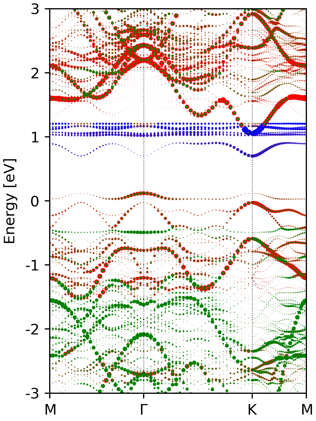
In the above script, we also superimpose the atomic contribution of each atoms to the states on the unfolded band plot. These lines get the atomic contributions of the selected atoms.
1
2
3
4
5
6
7
8
p = procar()
# The atomic contribution of Ce, Mo, S to each KS states
# index starting from 0
atomic_whts = [
    p.get_pw(0)[:,kmap,:],
    p.get_pw("1:18")[:,kmap,:],
    p.get_pw("18:54")[:,kmap,:]
]
Where the index of Ce, Mo and S atoms is 0 (the first atom), 2 to 18 and 19 to 54, respectively. If you do not want this, just comment out lines 43-54 and 64-65.
After executing the script, you should get a figure named ebs_s.png, which
looks like this.
The complete input files for the NSCF step and postprocessing can be downloaded here.