Schematics of e-ph Matrix in Wannier Representation
I was reading this article on electron-phonon interaction using Wannier functions when I noticed that Fig. 2 therein looks very simple and that I might be able to reproduce it using LaTeX/TikZ.

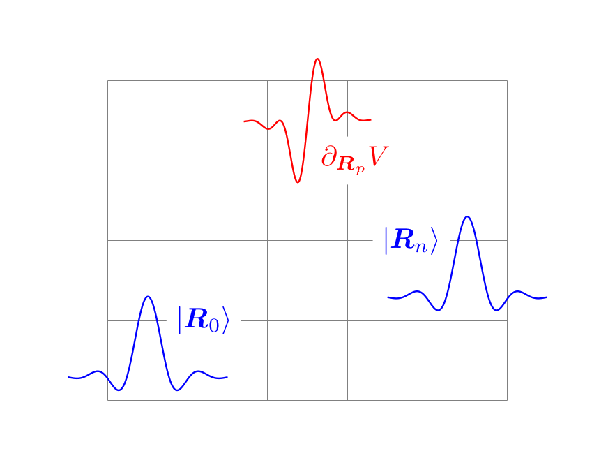
After carefully inspection of the figure, it seems that the Wannier function can by represented by
\[\begin{equation} W_n(x) = {\sin(\omega x) \over \alpha x}\cdot e^{-x^2/\beta} \end{equation}\]and the phonon perturbation $\partial_{R_p} V$ by
\[\begin{equation} \partial_{R_p} V = \gamma\cdot{\sin(\omega x)^2 \over \alpha x}\cdot e^{-x^2/\beta} \end{equation}\]Assuming that the grid space is $1$, we will limit the domain of $x$ to be $[-1,1]$.
Step to step plotting
First, load the necessary packages
\usepackage{braket}for Dirac bra/ket notation\usepackage{mathtools}for bold math symbols\usepackage{tikz}the main package for plotting
As a second step, draw the background grid. Here, the lower left corner of the
grid is (0, 0). The grid size is $5\times4$, the same as in the article.
1
\draw[gray, help lines, step=1] (0, 0) grid (5, 4);
Then, draw the Wannier functons. Here, we put the \draw command within the
scope environment so that we do NOT need to change the form of the Wannier
function when we want to plot another one in another cell. The only thing we
need to do is to set the center of the Wannier function by changing the shift
parameter of the \draw command.
1
2
3
4
5
6
7
8
9
10
11
12
13
\begin{scope}
  \draw[shift={(0.5, 0.3)}, line width=0.6pt, color=blue] plot [domain=-1:1, samples=300] (
      \x,
      {sin(12*\x r) / (\x*12) * exp(-\x*\x / 0.6)}
  );
\end{scope}

\begin{scope}
  \draw[shift={(4.5, 1.3)}, line width=0.6pt, color=blue] plot [domain=-1:1, samples=300] (
      \x,
      {sin(12*\x r) / (\x*12) * exp(-\x*\x / 0.6)}
  );
\end{scope}
In the same manner, we plot the phonon perturbation function.
1
2
3
4
5
6
\begin{scope}
  \draw[shift={(2.5, 3.5)}, line width=0.6pt, color=red] plot [domain=-0.8:0.8, samples=300] (
      \x,
      {1.5 * sin(9*\x r)*sin(9*\x r) / (\x*12) * exp(-\x*\x / 0.3)}
  );
\end{scope}
All the parameters of the function are fine tuned to best mimic the original figure.
As the last step, add some annotations.
1
2
3
4
5
6
7
8
9
\node [fill=white, blue] at (1.2, 1) {
  $\ket{\boldsymbol{R}_0}$
};
\node [fill=white, blue] at (3.8, 2) {
  $\ket{\boldsymbol{R}_n}$
};
\node [fill=white, red] at (3.1, 3) {
  $\partial_{\boldsymbol{R}_p} V$
};
Sometimes, you might want to change the size of the figure. To do this, put the
figure inside the \resizebox command.
The final code and result
Below is the complete LaTeX code:
1
2
3
4
5
6
7
8
9
10
11
12
13
14
15
16
17
18
19
20
21
22
23
24
25
26
27
28
29
30
31
32
33
34
35
36
37
38
39
40
41
42
43
44
\documentclass[border=20pt]{standalone}
\usepackage{braket}
\usepackage{mathtools}
\usepackage{tikz}

\begin{document}

\resizebox{0.50\textwidth}{!}{
  \begin{tikzpicture}
    \draw[gray, help lines, step=1] (0, 0) grid (5, 4);

    \begin{scope}
      \draw[shift={(0.5, 0.3)}, line width=0.6pt, color=blue] plot [domain=-1:1, samples=300] (
          \x,
          {sin(12*\x r) / (\x*12) * exp(-\x*\x / 0.6)}
      );
    \end{scope}
    \begin{scope}
      \draw[shift={(4.5, 1.3)}, line width=0.6pt, color=blue] plot [domain=-1:1, samples=300] (
          \x,
          {sin(12*\x r) / (\x*12) * exp(-\x*\x / 0.6)}
      );
    \end{scope}

    \begin{scope}
      \draw[shift={(2.5, 3.5)}, line width=0.6pt, color=red] plot [domain=-0.8:0.8, samples=300] (
          \x,
          {1.5 * sin(9*\x r)*sin(9*\x r) / (\x*12) * exp(-\x*\x / 0.3)}
      );
    \end{scope}

    \node [fill=white, text=blue] at (1.2, 1) {
      $\ket{\boldsymbol{R}_0}$
    };
    \node [fill=white, text=blue] at (3.8, 2) {
      $\ket{\boldsymbol{R}_n}$
    };
    \node [fill=white, text=red] at (3.1, 3) {
      $\partial_{\boldsymbol{R}_p} V$
    };
  \end{tikzpicture}
}

\end{document}
and the resulting figure: