Introduction
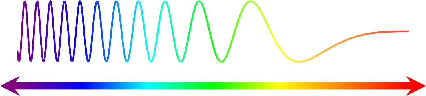
In this post, I will try to plot laser pulse using different methods. A laser pulse is often represented by a sine/cosine function multiplied by an envelope function, e.g. Gaussian
\[\begin{equation} f(t) = a \cdot \sin(\omega\cdot t) \cdot e^{-t^2/\tau^2} \end{equation}\]where $a$, $\omega$ and $\tau$ denotes the amplitude, frequency and duration of the laser pulse.
There are many tools that can be used to plot this function, e.g. gnuplot,
matplotlib. However, these tools are not convenient if you want to add an
arrow to the end of the laser pulse.
2D laser pulses using LaTeX TikZ
TikZ/LaTeX is convenient if you want to add arrows to the picture. Moreover, the
resulting picture is in pdf format, which is one of the vector images formats.
Below is the code that I used to generate the laser pulse.
1
2
3
4
5
6
7
8
9
10
11
12
13
14
15
16
17
\documentclass[border=20pt]{standalone}
\usepackage{tikz}
\usetikzlibrary{
  arrows,
  arrows.meta
}
\begin{document}

\resizebox{4in}{!}{
  \begin{tikzpicture}
    \draw[-{Stealth[length=20pt, open]}, line width=2.0pt, red]
    plot [samples=2000, domain=-6.5:6.5]
    (\x, {4*sin(\x r * 8) * exp(-\x*\x / 5.0)}) -- ++(0.5, 0);
  \end{tikzpicture}
}

\end{document}
Here is the result:

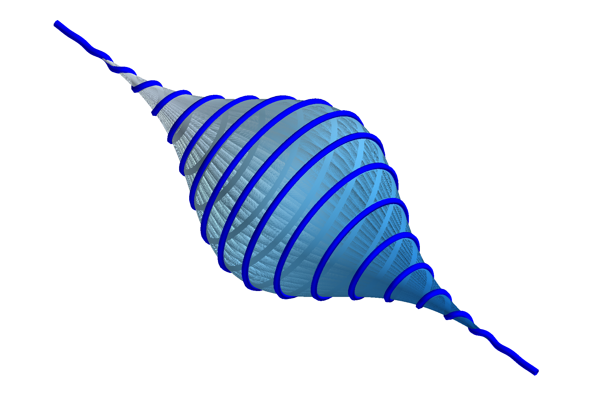
3D laser pulse using Mayavi
A 3D laser pulse is often much fancier than a 2D one. Function of 3d laser pulse
\[\begin{align} x &= a \cdot sin(\omega\cdot t) \cdot e^{-t^2 /\tau^2} \\ y &= a \cdot sin(\omega\cdot t) \cdot e^{-t^2 /\tau^2} \\ z &= c\cdot t \end{align}\]Mayavi can be used to plot a 3D one, as shown below.
1
2
3
4
5
6
7
8
9
10
11
12
13
14
15
16
17
18
19
20
21
22
23
24
25
26
27
28
29
30
31
32
33
34
35
36
37
#!/usr/bin/env python

import numpy as np
from mayavi import mlab

fig = mlab.figure(
    fgcolor=(0, 0, 0),
    bgcolor=(1, 1, 1),
    size=(2000, 2000)
)
fig.scene.parallel_projection = True

u = np.linspace(0, 2*np.pi, 1000)
v = np.linspace(-8, 8, 1000)

x = 2.5 * np.exp(-v**2 / 10) * np.sin(20*u)
y = 2.5 * np.exp(-v**2 / 10) * np.cos(20*u)
z = v

mlab.plot3d(x, y, z, tube_radius=0.09, color=(0, 0, 1))

u, v = np.mgrid[0:np.pi*2:1000j, -8:8:1000j]
x = 2.48 * np.exp(-v**2 / 10) * np.sin(20*u)
y = 2.48 * np.exp(-v**2 / 10) * np.cos(20*u)
z = v
mlab.mesh(x, y, z,
          # color=np.exp(-np.linspace(-8, 8, 1000)**2/10),
          colormap='Blues',
	  resolution=20,
          representation='surface',
          line_width=0,
          # tube_radius=0,
          # tube_sides=10,
          opacity=0.9)

# mlab.savefig('mlaser.png')
mlab.show()
After choosing the right view angle, one can get images like