
Introduction
The first Brillouin Zone (BZ) is the Wigner-Seitz cell of the reciprocal lattice, which can be constructed by applying Voronoi decomposition to a lattice.
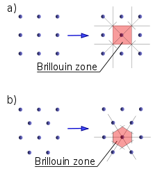
The reciprocal lattices (dots) and corresponding first Brillouin zones of (a) square lattice and (b) hexagonal lattice.
Constructing the Brillouin Zone
Below is the code that utilize scipy to generate the information of the BZ.
1
2
3
4
5
6
7
8
9
10
11
12
13
14
15
16
17
18
19
20
21
22
23
24
25
26
27
28
29
30
31
32
33
34
35
36
37
38
39
40
41
42
43
44
45
#!/usr/bin/env python

import numpy as np

def get_brillouin_zone_3d(cell):
    """
    Generate the Brillouin Zone of a given cell. The BZ is the Wigner-Seitz cell
    of the reciprocal lattice, which can be constructed by Voronoi decomposition
    to the reciprocal lattice.  A Voronoi diagram is a subdivision of the space
    into the nearest neighborhoods of a given set of points.

    https://en.wikipedia.org/wiki/Wigner%E2%80%93Seitz_cell
    https://docs.scipy.org/doc/scipy/reference/tutorial/spatial.html#voronoi-diagrams
    """

    cell = np.asarray(cell, dtype=float)
    assert cell.shape == (3, 3)

    px, py, pz = np.tensordot(cell, np.mgrid[-1:2, -1:2, -1:2], axes=[0, 0])
    points = np.c_[px.ravel(), py.ravel(), pz.ravel()]

    from scipy.spatial import Voronoi
    vor = Voronoi(points)

    bz_facets = []
    bz_ridges = []
    bz_vertices = []

    # for rid in vor.ridge_vertices:
    #     if( np.all(np.array(rid) >= 0) ):
    #         bz_ridges.append(vor.vertices[np.r_[rid, [rid[0]]]])
    #         bz_facets.append(vor.vertices[rid])

    for pid, rid in zip(vor.ridge_points, vor.ridge_vertices):
        # WHY 13 ????
        # The Voronoi ridges/facets are perpendicular to the lines drawn between the
        # input points. The 14th input point is [0, 0, 0].
        if(pid[0] == 13 or pid[1] == 13):
            bz_ridges.append(vor.vertices[np.r_[rid, [rid[0]]]])
            bz_facets.append(vor.vertices[rid])
            bz_vertices += rid

    bz_vertices = list(set(bz_vertices))

    return vor.vertices[bz_vertices], bz_ridges, bz_facets
The python function above returns the vertices, edges and facets of the BZ given the reciprocal basis vectors.
For an fcc lattice, the real-space basis vectors are defined by
1
2
3
cell = np.array([[0.0, 0.5, 0.5],
                 [0.5, 0.0, 0.5],
                 [0.5, 0.5, 0.0]])
For convenience, we have set the length of basis vectors to be 1.0.
The reciprocal lattice basis vectors and lengths can then be obtained
1
2
3
4
5
# basis vectors of the reciprocal lattice
icell = np.linalg.inv(cell).T

# length of the basis vectors
b1, b2, b3 = np.linalg.norm(icell, axis=1)
The vertices, edges and facets of the BZ
1
v, e, f = get_brillouin_zone_3d(cell)
Plotting the Brillouin Zone
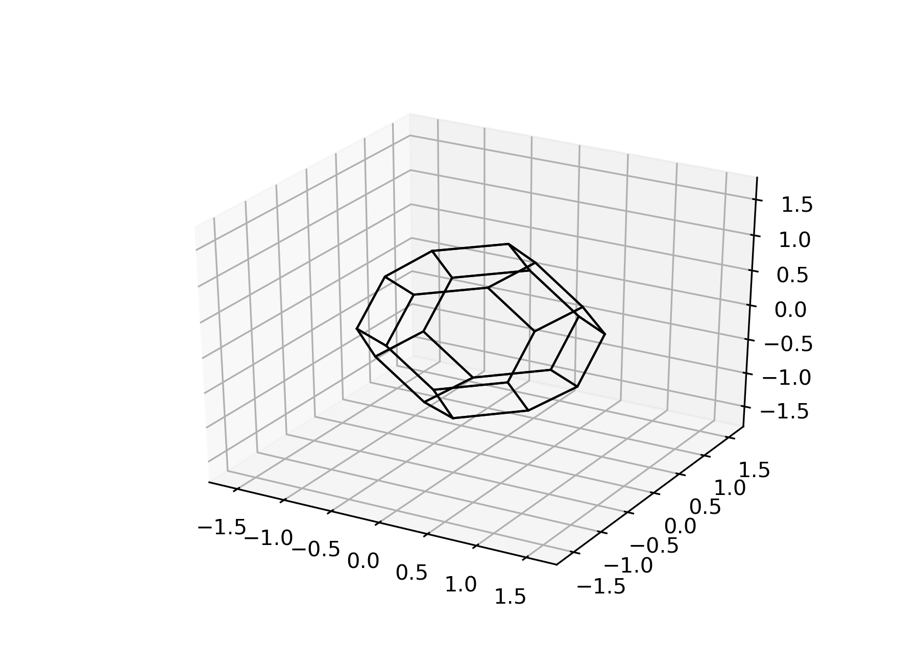
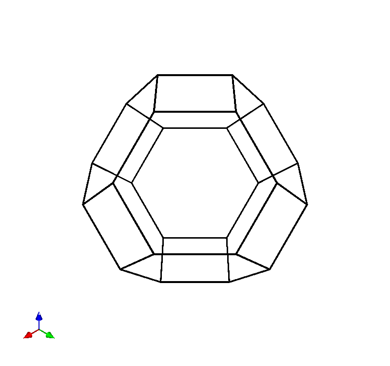
Once we have the information of the BZ, we can proceed to plot the Brillouin
Zone either using Matplotlib or Mayavi.
Matplotlib
1
2
3
4
5
6
7
8
9
10
11
12
13
14
15
16
17
import matplotlib.pyplot as plt
from mpl_toolkits.mplot3d import Axes3D

fig = plt.figure(
    figsize=(6, 6), dpi=300
)
ax = plt.subplot(111, projection='3d')
# ax = fig.add_subplot(111, projection='3d')

for xx in e:
    ax.plot(xx[:, 0], xx[:, 1], xx[:, 2], color='k', lw=1.0)

ax.set_xlim(-b1, b1)
ax.set_ylim(-b2, b2)
ax.set_zlim(-b3, b3)

plt.show()
Mayavi
1
2
3
4
5
6
7
8
9
10
11
12
13
14
15
from mayavi import mlab
fig = mlab.figure(
    bgcolor=(1, 1, 1),
    size=(800, 800)
)

bz_line_width = b1 / 200

for xx in e:
    mlab.plot3d(xx[:, 0], xx[:, 1], xx[:, 2],
                tube_radius=bz_line_width,
                color=(0, 0, 0))

mlab.orientation_axes()
mlab.show()
The full code can be found here.