
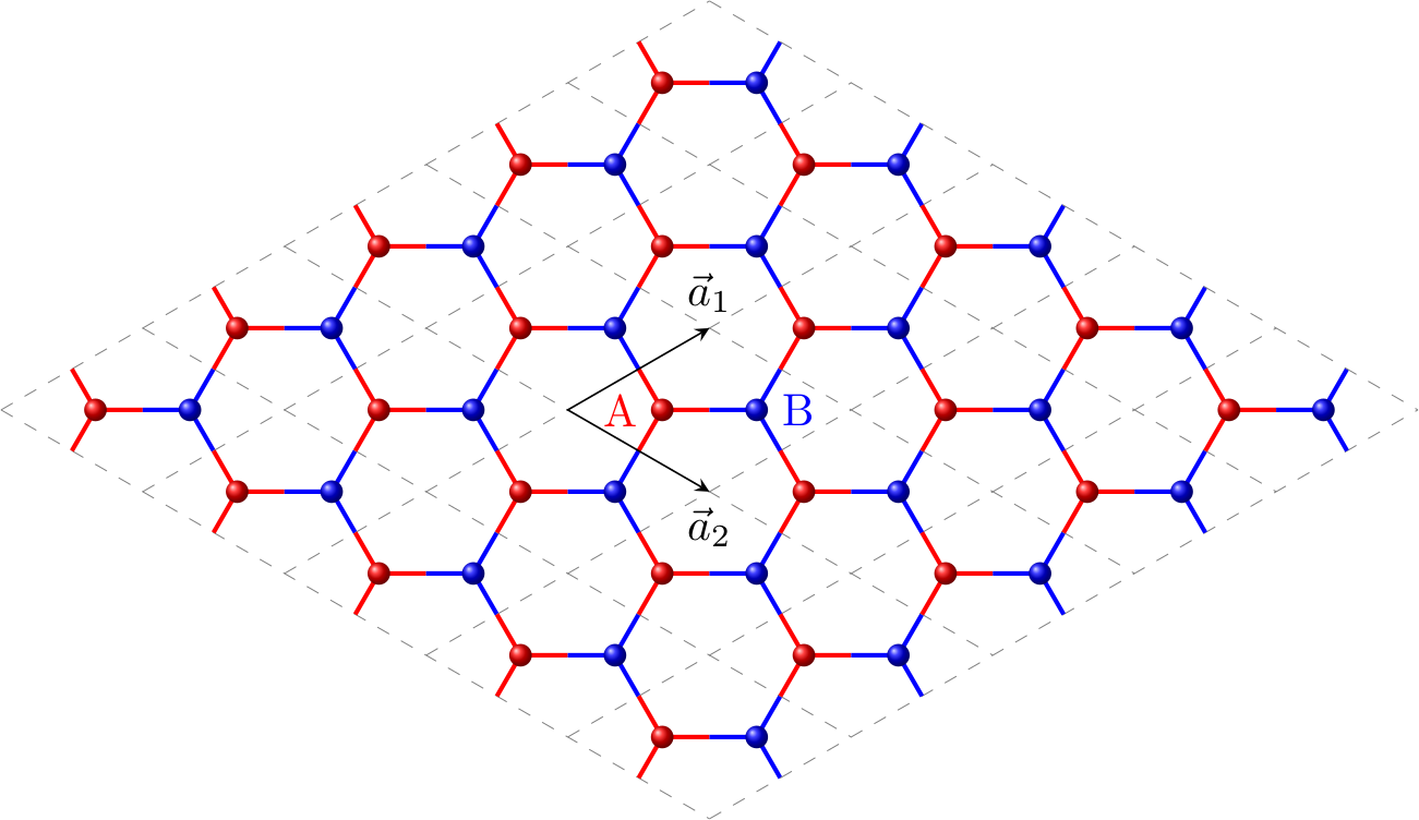
Honeycomb lattice of graphene
The unit cell of graphene’s lattice consists of two different types of sites, which we will refer to as $A$ and $B$ sites (see Figure 1).
With the basis vectors, the cell can be defined by the cell vector
\[\begin{equation} \boldsymbol{R}_n = j\cdot\vec{a}_1 + k\cdot\vec{a}_2 \end{equation}\]Below we will used $(j, k)$ to denote the cell index.
Nearest-neighbour Tighting Binding Model for Graphene
The Hamiltonian of the graphene lattice
\[\begin{equation} {\hat H} = -\frac{\hbar^2}{2m}\nabla^2 + U(\boldsymbol{r}) \end{equation}\]where $U(\boldsymbol{r})$ is the periodic potential of the crystal. The Schrödinger equation follows
\[\begin{equation} \left[ -\frac{\hbar^2}{2m}\nabla^2 + U(\boldsymbol{r}) \right] \psi_{\boldsymbol{k}}(\boldsymbol{r}) = E(\boldsymbol{k}) \psi_{\boldsymbol{k}}(\boldsymbol{r}) \end{equation}\]where $\psi_{\boldsymbol{k}}(\boldsymbol{r})$ is the wavefunction of the electron, and $E(\boldsymbol{r})$ is the corresponding energy.
Assuming that $w_\alpha(\boldsymbol{r} - \boldsymbol{R}_n)$ are orthonormal wavefunctions located at site $\alpha$ of the cell $\boldsymbol{R}_n$, i.e.
\[\begin{equation} \int_V\, w^*_\alpha(\boldsymbol{r} - \boldsymbol{R}_n) w_\beta(\boldsymbol{r} - \boldsymbol{R}_m) \, \mathrm{d}\boldsymbol{r} = \delta_{\alpha\beta} \delta_{mn} \end{equation}\]According to the Bloch’s theorem, the wavefunction of the electron in a periodic potential can be written as linear combination of the Bloch sum, i.e.
\[\begin{equation} \psi_{\boldsymbol{k}}(\boldsymbol{r}) = \frac{1}{\sqrt{N}}\sum_\alpha C_\alpha(\boldsymbol{k}) \sum_n e^{i\boldsymbol{k}\cdot\boldsymbol{R}_n} w_\alpha(\boldsymbol{r} - \boldsymbol{R}_n) \end{equation}\]By expanding the Hamiltonian in the Bloch sum basis, we have
\[\begin{equation} H(\boldsymbol{k}) = \begin{bmatrix} H_{11} & H_{12} \\ H_{21} & H_{22} \end{bmatrix} \end{equation}\]where $H_{\alpha\beta}$ is given by
\[\begin{align} H_{\alpha\beta} &= \frac{1}{N} \sum_{nm} \int_V\, e^{i\boldsymbol{k}\cdot(\boldsymbol{R}_m - \boldsymbol{R}_n)}\, w^*_\alpha(\boldsymbol{r} - \boldsymbol{R}_n) \, {\cal H}(\boldsymbol{r}) \, w_\beta(\boldsymbol{r} - \boldsymbol{R}_m) \, \mathrm{d}\boldsymbol{r} \nonumber \\[6pt] &= \sum_n \int_V\, e^{i\boldsymbol{k}\cdot\boldsymbol{R}_n}\, w^*_\alpha(\boldsymbol{r} - \boldsymbol{R}_n) \, {\cal H}(\boldsymbol{r}) \, w_\beta(\boldsymbol{r} - \boldsymbol{R}_0) \, \mathrm{d}\boldsymbol{r} \cr \end{align}\]where we used the fact that the integrand only depends on the distance between the site $\boldsymbol{R}_n$ and $\boldsymbol{R}_m$.
In the nearest-neighbours tight-binding model, we only considter those terms with $ | n | \le 1 $.
The diagonal matrix elements
Apparently, only $n=0$ contributes to the matrix elements $H_{11}$ and $H_{22}$, therefore
\[\begin{align} H_{11} = H_{22} &= \int_V\, w^*_1(\boldsymbol{r} - \boldsymbol{R}_0) \, {\cal H}(\boldsymbol{r}) \, w_1(\boldsymbol{r} - \boldsymbol{R}_0) \, \mathrm{d}\boldsymbol{r} \nonumber \\[6pt] &= \int_V\, w^*_2(\boldsymbol{r} - \boldsymbol{R}_0) \, {\cal H}(\boldsymbol{r}) \, w_2(\boldsymbol{r} - \boldsymbol{R}_0) \, \mathrm{d}\boldsymbol{r} \nonumber \\[6pt] &= \varepsilon_0 \end{align}\]The off-diagonal matrix elements
Let’s first inspect the $H_{12}$ term. One can see from Figure 1 that the nearest-neighbours of the $A$ site in cell $(j, k)$ located in the cell $(j, k$), $(j-1, k)$ and $(j, k-1)$, respectively. As a result, the $H_{12}$ term can be readily written.
\[\begin{align} H_{12} &= \int_V\, w^*_1(\boldsymbol{r} - \boldsymbol{R}_0) \, {\cal H}(\boldsymbol{r}) \, w_2(\boldsymbol{r} - \boldsymbol{R}_0) \, \mathrm{d}\boldsymbol{r} \nonumber\\[6pt] &+ e^{-i\boldsymbol{k}\cdot\boldsymbol{a}_1}\, \int_V\, w^*_1(\boldsymbol{r} - \boldsymbol{R}_{(-1, 0)}) \, {\cal H}(\boldsymbol{r}) \, w_2(\boldsymbol{r} - \boldsymbol{R}_0) \, \mathrm{d}\boldsymbol{r} \nonumber \\[6pt] &+ e^{-i\boldsymbol{k}\cdot\boldsymbol{a}_2}\, \int_V\, w^*_1(\boldsymbol{r} - \boldsymbol{R}_{(0, -1)}) \, {\cal H}(\boldsymbol{r}) \, w_2(\boldsymbol{r} - \boldsymbol{R}_0) \, \mathrm{d}\boldsymbol{r} \end{align}\]By further assuming that the integral of the last three terms are the same, i.e.
\[\begin{equation} t = \int_V\, w^*_1(\boldsymbol{r} - \boldsymbol{R}_0) \, {\cal H}(\boldsymbol{r}) \, w_2(\boldsymbol{r} - \boldsymbol{R}_0) \, \mathrm{d}\boldsymbol{r} \end{equation}\]we have
\[\begin{equation} H_{12} = t\left[ 1 + e^{-i\boldsymbol{k}\boldsymbol{a}_1} + e^{-i\boldsymbol{k}\boldsymbol{a}_2} \right] \end{equation}\]Similarly, we have
\[\begin{equation} H_{21} = t\left[ 1 + e^{i\boldsymbol{k}\boldsymbol{a}_1} + e^{i\boldsymbol{k}\boldsymbol{a}_2} \right] \end{equation}\]The complete matrix
Putting together all the matrix element, we have
\[\begin{equation} H(\boldsymbol{k}) = \begin{bmatrix} \varepsilon_0 & t\left[ 1 + e^{-i\boldsymbol{k}\boldsymbol{a}_1} + e^{-i\boldsymbol{k}\boldsymbol{a}_2} \right] \\ t\left[ 1 + e^{i\boldsymbol{k}\boldsymbol{a}_1} + e^{i\boldsymbol{k}\boldsymbol{a}_2} \right] & \varepsilon_0 \end{bmatrix} \end{equation}\]The eigenvalues $E(\boldsymbol{k})$ can then be easily obtained
\[\begin{align} E(\boldsymbol{k}) &= \varepsilon_0 \pm t\sqrt{ 1 + e^{-i\boldsymbol{k}\boldsymbol{a}_1} + e^{ i\boldsymbol{k}\boldsymbol{a}_1} + e^{-i\boldsymbol{k}\boldsymbol{a}_2} + e^{ i\boldsymbol{k}\boldsymbol{a}_2} + (e^{-i\boldsymbol{k}\boldsymbol{a}_1} + e^{-i\boldsymbol{k}\boldsymbol{a}_2}) (e^{ i\boldsymbol{k}\boldsymbol{a}_1} + e^{ i\boldsymbol{k}\boldsymbol{a}_2}) } \nonumber \\[6pt] &= \varepsilon_0 \pm t\sqrt{ 3 + 2\cos(\boldsymbol{k}\boldsymbol{a}_1) + 2\cos(\boldsymbol{k}\boldsymbol{a}_2) + 2\cos(\boldsymbol{k}(\boldsymbol{a}_1-\boldsymbol{a}_2)) } \end{align}\]One of the definitions for the hexagonal lattice is
\[\begin{align} \vec{a}_1 &= {a\over2}(3, \sqrt{3}) \\[6pt] \vec{a}_2 &= {a\over2}(3,-\sqrt{3}) \end{align}\]where $a$ is the bond-length of the graphene. With this definition, the energy band of graphene follows.
\[\begin{equation} E_(k_x, k_y) = \pm t \sqrt{ 3 + 2 \cos(\sqrt{3}k_y a) + 4 \cos({3\over2}k_x a)\cos({\sqrt{3}\over2}k_y a) } \end{equation}\]Generated by Plotly