In this training session, we will learn how to do an NAMD calculation using Hefei-NAMD.
Outline of the session:
A bit of theory
Fewest-Switches Surface Hopping
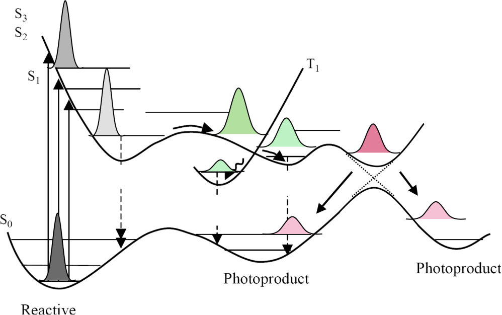
Surface hopping is a mixed quantum-classical technique that incorporates quantum mechanical effects into molecular dynamics simulations. Traditional molecular dynamics assume the Born-Oppenheimer approximation, where the lighter electrons adjust instantaneously to the motion of the nuclei. Though the Born-Oppenheimer approximation is applicable to a wide range of problems, there are several applications, such as photoexcited dynamics, electron transfer, and surface chemistry where this approximation falls apart. Surface hopping partially incorporates the non-adiabatic effects by including excited adiabatic surfaces in the calculations, and allowing for ‘hops’ between these surfaces, subject to certain criteria. One of the most famous criteria is the so-called fewest-switches algorithm proposed by John C. Tully, which minimizes the number of hops required to maintain the population in various adiabatic states.
In the mixed quantum-classical method, electrons are treated as quantum subsystem and evolves according to the time-dependent Schrödinger equation
\[\begin{equation} i\hbar \frac{ \partial\Phi(\mathbf{r}, \mathbf{R}, t) }{ \partial t } = {\hat{\cal H}}_{el}(\mathbf{r}, \mathbf{R}) \Phi(\mathbf{r}, \mathbf{R}, t) \end{equation}\]We then expand the wavefunction $\Phi(\mathbf{r}, \mathbf{R}, t)$ in a basis , $\Psi_j(\mathbf{r}, \mathbf{R})$.
\[\begin{equation} \Phi(\mathbf{r}, \mathbf{R}, t) = \sum_j C_j(t)\Psi_j(\mathbf{r}, \mathbf{R}) \end{equation}\]In most applications, the basis functions are selected as the eigenfunctions of ${\hat{\cal H}}_{el}(\mathbf{r}, \mathbf{R})$, which is also referred to as the adiabatic representation. Other basis or representation can also be used in the above formulation. Substituting the above equation into the time dependent Schrödinger equation gives
\[\begin{equation} i\hbar\dot C_j(t) = \sum_k C_k(t) \left[H_{jk} - i\hbar\mathbf{\dot R}\cdot \mathbf{d}_{jk} \right] \end{equation}\]Where $H_{jk}$ and the nonadiabatic coupling vector $\mathbf{d}_{jk}$ are given by
\[\begin{align} H_{jk} &= \langle \Psi_j | {\hat{\cal H}}_{el} | \Psi_k \rangle \\ \mathbf{d}_{jk} &= \langle \Psi_j | \nabla_{\mathbf{R}} | \Psi_k \rangle \end{align}\]
The nuclei in the mixed quantum-classical medthod are treated as classical particles and follow the Newton’s equation. Surface hopping and Ehrenfest dynamics differ in the way how this is done: the nuclei evolve on a single potential energy surface at any given moment in surface hopping while on an averaged potential energy surface in Ehrenfest dynamics. The trajectories are allowed to hop between the potential energy surface in surface hopping. In the most famous fewest-switches algorithm, the hops can happen at any moment and the hopping probability bewteen the potential energy surface is given by
\[\begin{equation} P_{jk}(t,\Delta t)=\max\Biggl( -\frac{ 2\int_t^{t + \Delta t}\mathrm{d}{t}\left[ \hbar^{-1} \Im(\rho_{jk} H_{jk}) - \Re(\rho_{jk}\mathbf{d}_{jk}\cdot\mathbf{\dot R}) \right] }{ \rho_{jj} } ,\,0\, \Biggr) \end{equation}\]FSSH + TDDFT
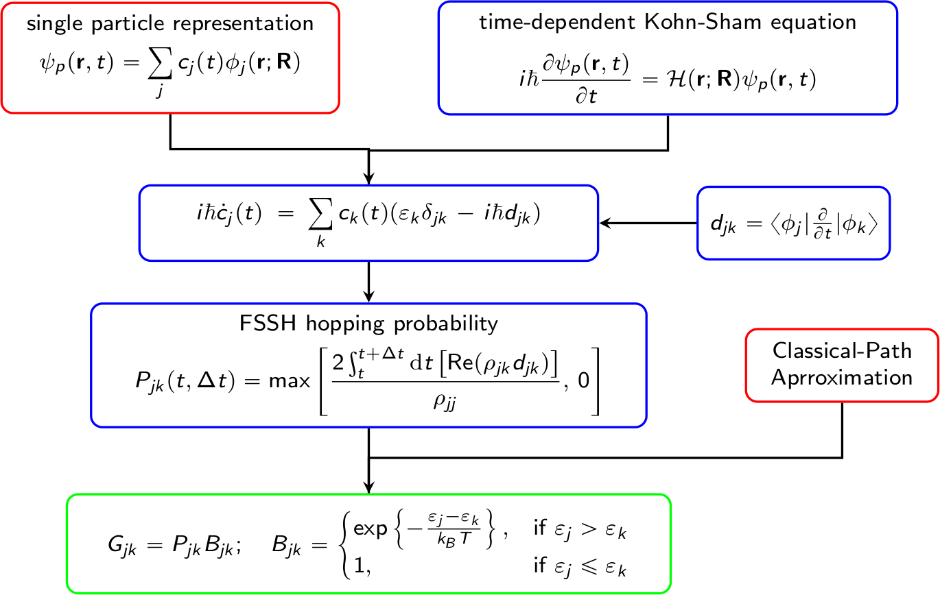
A brief flowchart of Hefei-NAMD
-
Build a supercell of investigated system and perform the geometry optimization at 0 K.
-
Starting with the optimized structure, perform ab initio molecular dynamics and obtain a MD trajectory.
-
Extract snapshots from the MD trajectory and perform SCF calculation for each of the snapshots.
-
Read WAVECAR in step 3 and perform NAMD.
-
Analyze the results.

reference
-
“Ab initio nonadiabatic molecular dynamics investigations on the excited carriers in condensed matter systems”, Wiley Interdisciplinary Reviews: Computational Molecular Science, 9, e1411
-
“Molecular dynamics with electronic transitions”, J. Chem. Lett., 93(2): 1061–1071.
-
“Trajectory Surface Hopping in the Time-Dependent Kohn-Sham Approach for Electron-Nuclear Dynamics”, Phys. Rev. Lett., 95, 163001
Installation
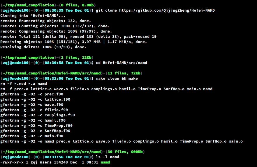
Hefei-NAMD is mainly written in Fortran and barely depends on any third-party library. The compilation of Hefei-NAMD is very simple, all you need is a FORTRAN compiler. On your linux shell, do the following steps:
-
get the source code:
1
git clone https://github.com/QijingZheng/Hefei-NAMD
-
change to the source code directory
1
cd Hefei-NAMD/src/namd
Note that under the
src/directory, there are three sub-directories. For the moment, we will concentrate on the above one. -
Just type
makeand you should have an executable namednamdin the current directory.
Figure 5. The compilation process of Hefei-NAMD.
In case you want to access the executable from anywhere in the system, just add
the path of the namd executable to the "PATH" environment variable, i.e.
1
cat 'export PATH=/path/to/your/namd-executable:${PATH}' >> ~/.bashrc
Learn Hefei-NAMD by an example
Below, we will go through the basic procedure of Hefei-NAMD, by investigating the photo-generated carrier dynamics at van der Waals TMD heterostructure intreface. This work was carried out by Mr. Yunzhe Tian (yunzhe@mail.ustc.edu.cn) and published on J. Phys. Chem. Lett., 11, 586−590(2020).
Ground state properties of the vdW heterostructure
Before doing NAMD calculations, it is always crucial to have a basic idea of the properties of the system you are about to investigate. For example, the geometry and electronic structures.
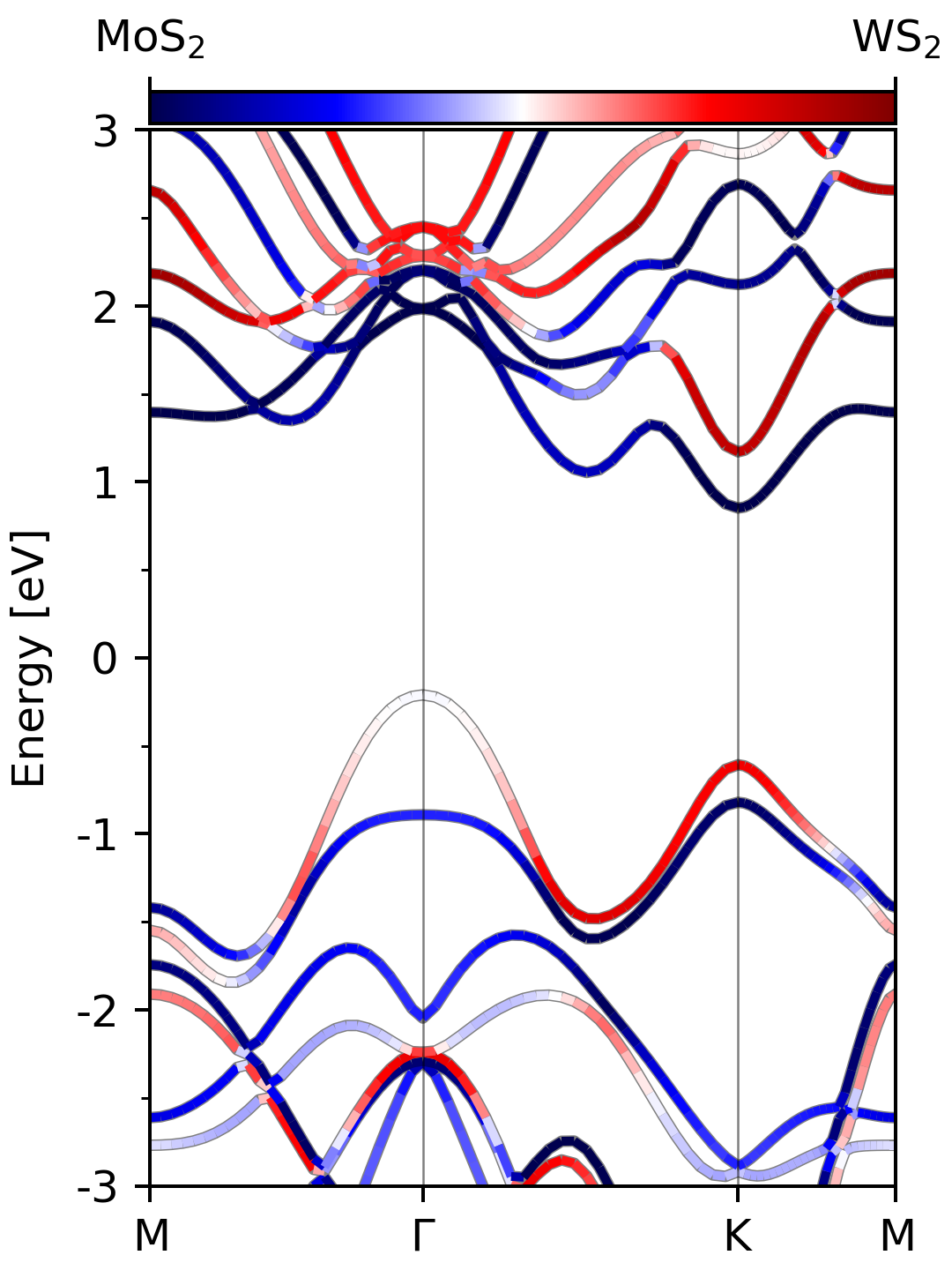
In the figure above, the band structure of the strain-free MoS$_2$/WS$_2$ heterostructure is shown. Incidently, the band strcuture can be easily obtained by using pyband. The command line to generate the above picture is
1
2
3
4
5
6
7
8
pyband  --occ '1 2 6' \                          # the atom index of WS2
        --occL \                                 # use the color stripes to plot the band
        --occLC_cmap seismic \                   # choose the colormap "seismic"
        --occLC_cbar_ticks '0 1' \               # set the color range from 0 to 1
        --occLC_cbar_vmin 0 \                    #
        --occLC_cbar_vmax 1 \                    #
        --occLC_cbar_ticklabels 'MoS$_2$ WS$_2$' # 0 corresponds to MoS2, 1 corresponds to WS2
        -k mgkm                                  # the name of the high-symmetry k-point
As can be clearly seen from the picture, the MoS$_2$/WS$_2$ vdW heterostructure is of type-II band alignment, where the CBM and VBM reside on different constituent TMD layers. Therefore, in this system, we can study the dynamics of photo-generated electron from WS$_2$ to MoS$_2$ or dynamics of photo-generated hole from MoS$_2$ to WS$_2$.
To achieve this, we first need to build a supercell. The supercell must conform to the following rules:
-
The supercell should be large enough, since the Brillouin Zone in all the calculation hereafter will be sampled only at $\Gamma$ point. Needless to say, the supercell should not be too large, too.
-
The shape or size of the supercell should be chosen carefully. The shape of the supercell is not uniquely defined. For example, in our case of MoS$_2$/WS$_2$ heterostructure, we can either choose a hexagonal supercell or a tetragonal supercell as was used in our paper. If you choose our supercell to be hexagonal, then only $3n\times 3n$ supercell should be chosen, since otherwise the $K$ point will not fold onto the $\Gamma$ point.
Once the supercell is determined, perform a geometry optimization and get the optimized structure. Note that Gammon-only version of VASP should be used to do the calculations, since we only sample the BZ by $\Gamma$-point and Gamma-only version of VASP will speed up the calculation by ~50%.
Ground state molecular dynamics
Now that we have the optimized structure, the next step is to obtain a molecular
dynamics trajectory. First, we need to do an equilibration molecular dynamics to
add thermal energy to the optimized structure. Below is an example VASP INCAR
file that uses the velocity-rescaling method (SMASS = -1) to bring the
temperature of the system to 300 K. The optimized structure in the last step is
used as the POSCAR file and the KPOINTS file only contains the $\Gamma$
point.
1
2
3
4
5
6
7
8
9
10
11
12
13
14
15
16
17
18
19
20
21
22
23
24
25
26
27
28
29
30
31
General
  SYSTEM  = Your Job Name
  PREC    = Med
  ISPIN   = 1
  ISTART  = 0
  ICHARG  = 1

Electronic relaxation
  NPAR    = 4
  ISMEAR  = 0
  SIGMA   = 0.1
  ALGO    = Fast
  NELMIN  = 4
  NELM    = 120
  EDIFF   = 1E-6

Molecular Dynamics
  ISYM    = 0     # turn off symmetry for MD
  IBRION  = 0     # turn on MD
  NSW     = 500   # No. of ionic steps
  POTIM   = 1     # time step 1.0 fs
  SMASS   = -1    # velocity rescaling
  NBLOCK  = 4     # velocity rescaled
                  # every NBLOCK step
  TEBEG   = 300   # start temperature
  TEEND   = 300   # end temperature

Writing Flag
  NWRITE  = 1     # make OUTCAR small
  LWAVE   = .FALSE.
  LCHARG  = .FALSE.
The temperature of the molecular dynamics is written in the OSZICAR file. Use
this simple script (vaspT) to plot the temperature
variationc curve.
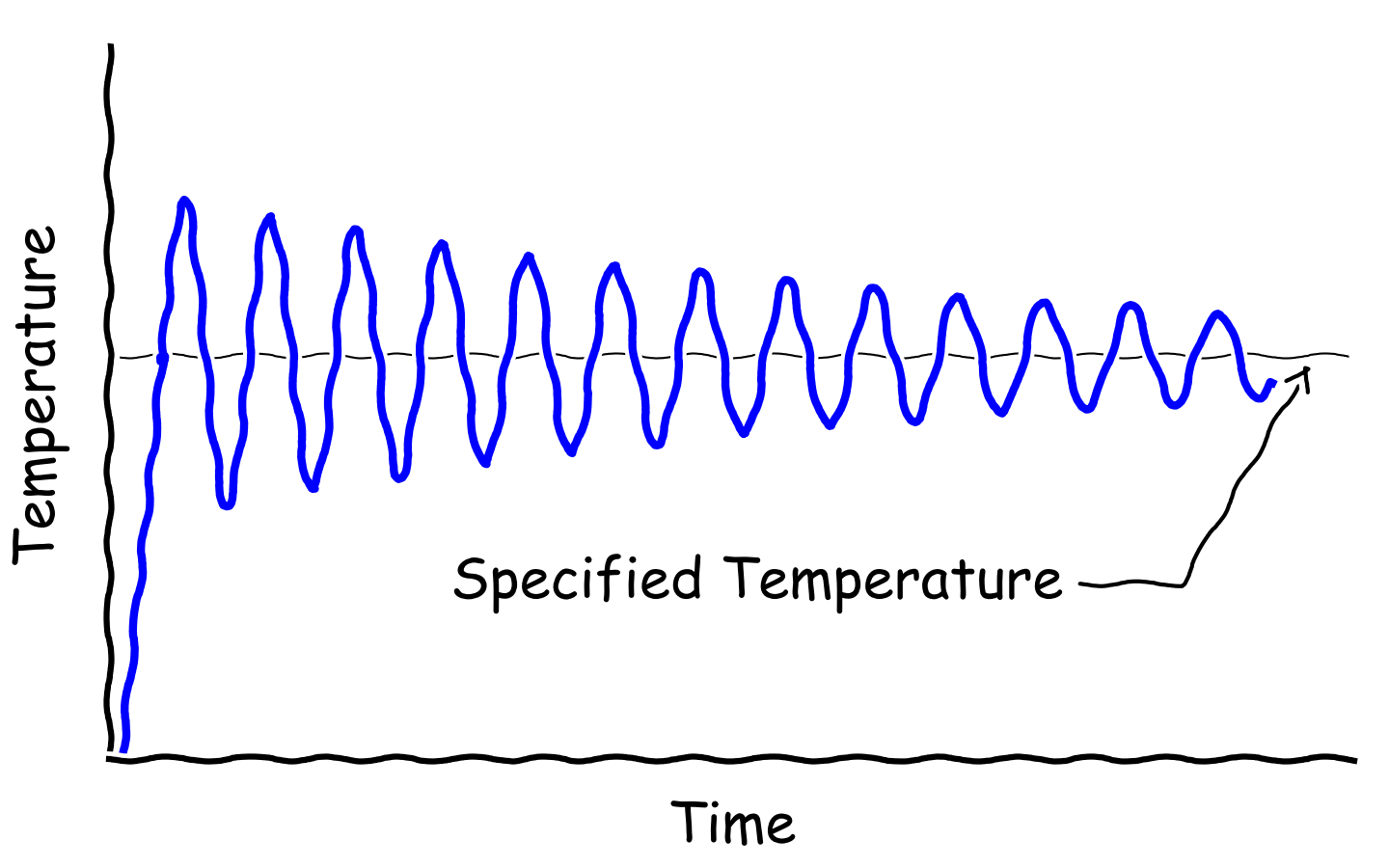
The temperature of the system behaves something like the picture above.
Initially, the temperature fluctuates drastically. As time goes by, the
amplitude of the fluctuation should become smaller and finally the temperature
should oscillate around the specified temperature (TEEND). A general rule of
thumb is that once the fluctuation is smaller than 10% of the expected
temperature, the system can be considered as being in equilibrium and the
calculation can be stopped.
-
Note that we have set
NSW = 500in the INCAR file. Sometimes, the system may not reach the equilibrium in one single run. As a result, you should make a new directory, copyCONTCARtoPOSCARand start another run. -
Another important parameter is the
POTIM, which is determined by the highest vibration frequency of the system. If there are light elements in your supercell, hydrogen for example, you might want to use a smallerPOTIM. -
After the system reaches equilibrium, have a look at the final structure
CONTCAR, make sure that the structure is OK. I have run into cases when the temperature looked good while the layer distance became too large, in a sense that they were more like two independent parts. In this case, you might want to try another algorithm, e.g.SMASS > 0.
Once the system reaches equilibrium, we can proceed to the next step: the
production MD. In this step, we run the MD with the microcanonical ensemble
(SMASS = -3), as is shown in the INCAR example below.
-
make another new directory and copy
CONTCARof last step asPOSCARof the current step. -
set
NBLOCK = 1inINCARto write every snapshot of the trajectory toXDATCAR, which we will need to extract the configurations. -
The
NSWdepends on the time scale of the problem you are investigating. For example, in our example of photo-generated carrier dynamics, the experimental time scale is about 100 fs, thenNSW = 5000is far more than enough. For processes that are generally much slower, e.g, the electron/hole recombination process, which might be of nanosecond scale,NSW = 5000might not be enough. We use another techinique to deal with this problem, which is not covered in the current session. -
In the microccanonical ensemble (NVE), the total energy is conserved, which can be used as a signature of the quality of the MD run. (See the third figure in the output of vaspT.
1
2
3
4
5
6
7
8
9
10
11
12
13
14
15
16
17
18
19
20
21
22
23
24
25
26
27
28
29
General
  SYSTEM  = Your Job Name
  PREC    = Med
  ISPIN   = 1
  ISTART  = 0
  ICHARG  = 1

Electronic relaxation
  NPAR    = 4
  ISMEAR  = 0
  SIGMA   = 0.1
  ALGO    = Fast
  NELMIN  = 4
  NELM    = 120
  EDIFF   = 1E-6

Molecular Dynamics
  ISYM    = 0     # turn off symmetry in MD
  IBRION  = 0     # MD flag
  NSW     = 5000  # NSW*POTIM fs
  POTIM   = 1     # time step 1.0 fs
  SMASS   = -3    # Microcanonical
  NBLOCK  = 1     # XDATCAR contains
                  # positions of each step

Writing Flag
  NWRITE  = 1       # make OUTCAR small
  LWAVE   = .FALSE. # WAVECAR not needed
  LCHARG  = .FALSE. # CHG not needed
SCF calculations
In this step, we will extract the nuclei positions at each time step from the MD trajectory and then perform SCF calculation for each one of them. We can do this with the help of a small python script, wihich utilize the Atomic Simulation Environment (ASE).
1
2
3
4
5
6
7
8
9
10
11
12
13
14
15
16
17
18
19
20
21
22
23
24
25
26
27
28
29
#!/usr/bin/env python

import os
from ase.io import read, write

# This may take a little while, since OUTCAR may be large for long MD run.
# CONFIGS = read('/path/to/OUTCAR', format='vasp-out', index=':')

################################################################################
# or you can read positions from XDATCAR, which is faster since it only contains
# the coordinates.  You may have to process the XDATCAR beforehand when VASP
# forget to write some lines. Executing the following line on shell prompt.
################################################################################
# for vasp version < 5.4, please execute the following command before the script
# sed -i 's/^\s*$/Direct configuration=/' XDATCAR
################################################################################
CONFIGS = read('example/nve/XDATCAR', format='vasp-xdatcar', index=':')

NSW    = len(CONFIGS)               # The number of ionic steps
NSCF   = 2000                       # Choose last NSCF steps for SCF calculations
NDIGIT = len("{:d}".format(NSCF))   #
PREFIX = 'example/waveprod/run/'    # run directories
DFORM  = "/%%0%dd" % NDIGIT         # run dirctories format
for ii in range(NSCF):              # write POSCARs
    p = CONFIGS[ii - NSCF]
    r = (PREFIX + DFORM) % (ii + 1)
    if not os.path.isdir(r): os.makedirs(r)
    write('{:s}/POSCAR'.format(r), p, vasp5=True, direct=True)
This script can read the MD trajectory from either OUTCAR or XDATCAR file.
Subsequently, the script saves the last NSCF (in this case 2000) snapshots as
VASP POSCAR files under the directory PREFIX (“./run” in this case). Modify
the script accordingly to fit your need before executing the script. When it
finishes, you should have 2000 directories named 0001/ to 2000/ under the
parent directory PREFIX.
The next step is to perform SCF calculations under these 2000 directories.
- Prepare
INCAR,KPOINTSandPOTCARunder thePREFIXdirectory. Create symbolic links in each sub-directory0001/to2000/using the followingbashfor-loop.
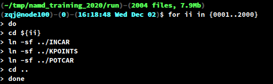
- The
INCARis just any ordinary SCFINCARexcept a few notes to the tags in theINCAR
1
2
3
4
5
6
7
    PREC = Accurate   # Precision large enough for accurte descripiton of the wavefunction
   EDIFF = 1E-6       # well converged electronic structure
   LWAVE = .TRUE.     # We need the WAVECARs
  NBANDS = xxx        # make sure we have the same number of bands.
                      # Also be large enough, since the last few bands are not very accurate.
  LORBIT = 11         # we will need PROCAR to analyze the results
    NELM = 120        # large enouth so that the electronic structure can converge the require precision
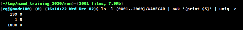
- After all the SCF calculations are finished, check that all
WAVECARs have the same size. We can do this with a small bash command line. As can be clearly seen in the output, the WAVECAR in0200has a different size.
NAMD calculations
Finally, we are in a position to start NAMD calculations.
First, check the time dependent Kohn-Sham energies from the previous SCF calculations. This can be done by another auxiliary script tdksen.py, with a little modificaiton.
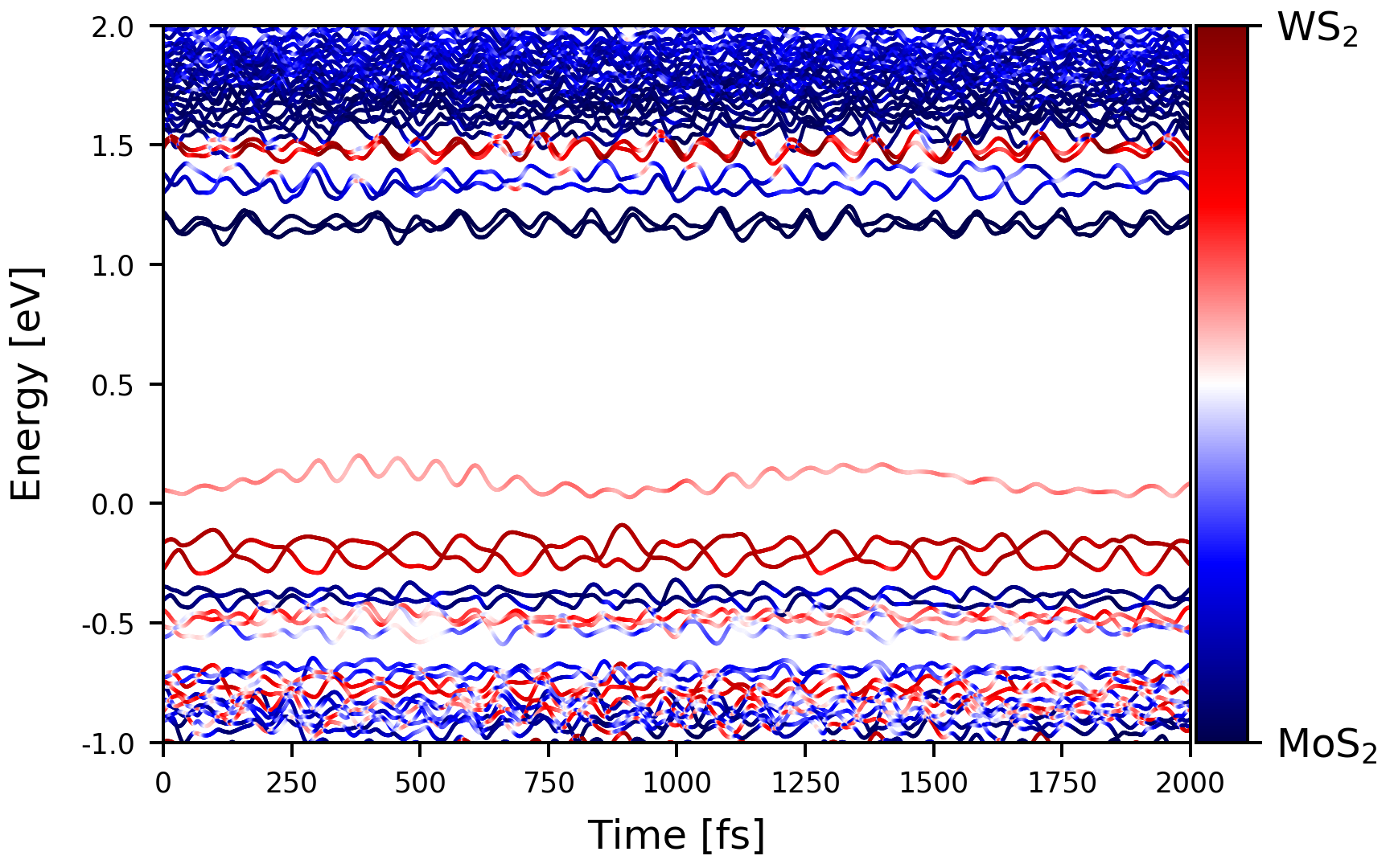
This script will read the energies and weight of selected atoms from the
PROCARs in the sub-directories 0001 to 2000. Moreover, these data will be
saved as all_en.npy and all_wht.npy so that on a second call of the script,
there is no need to read the PROCARs again. Below are some customized
parameters that need to be specified.
1
2
3
4
5
6
7
8
9
10
11
12
13
14
nsw     = 2000
dt      = 1.0
nproc   = 8
prefix  = 'waveprod/run/'
runDirs = [prefix + '/{:04d}'.format(ii + 1) for ii in range(nsw)]
# which spin, index starting from 0
whichS  = 0
# which k-point, index starting from 0
whichK  = 0
# which atoms, index starting from 0.
# In this case, the atomic index of WS2
whichA  = np.arange(54) + 54
Alabel  = r'WS$_2$'
Blabel  = r'MoS$_2$'
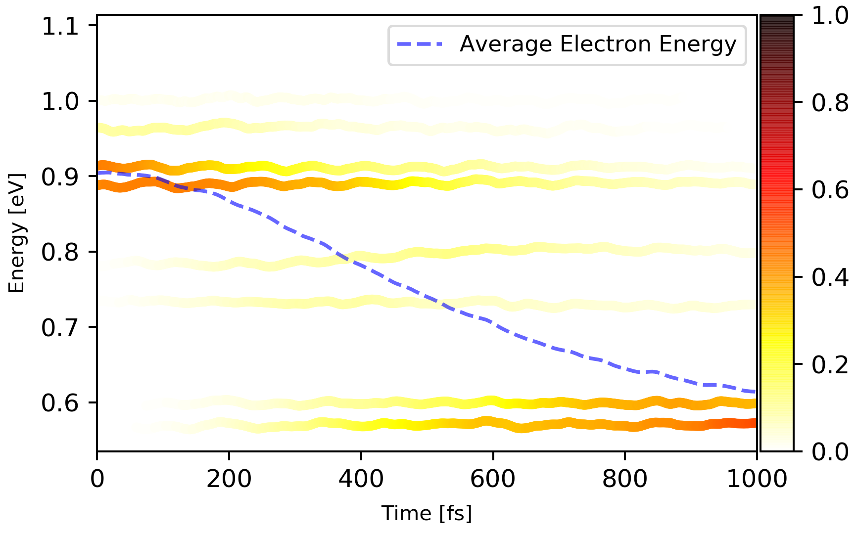
We will investigate the photo-generated electron transfer from WS$_2$ to MoS$_2$. The initial photoexcited electron is located at the conduction band contributed by WS$_2$ at about 1.5 eV. The hot electron will relax to the conduction band minimum.
To perform a NAMD calculation, we need two input files: inp and INICON.
-
inpcontains the input control parameters. -
INICONcontains the initial excited conditions.
Below is the inp file that we used:
1
2
3
4
5
6
7
8
9
10
11
12
13
14
15
16
17
18
&NAMDPARA
  BMIN     = 325     ! bottom band index, starting from 1
  BMAX     = 335     ! top band index
  NBANDS   = 388     ! number of bands

  NSW      = 2000    ! number of ionic steps
  POTIM    = 1       ! MD time step
  TEMP     = 300     ! temperature in Kelvin

  NSAMPLE  = 100     ! number of samples
  NAMDTIME = 1000    ! time for NAMD run
  NELM     = 1000    ! electron time step
  NTRAJ    = 5000    ! SH trajectories
  LHOLE    = .FALSE. ! hole/electron SH

  RUNDIR   = "waveprod/run/"
!  LCPEXT   = .TRUE.
/                    ! **DO NOT FORGET THE SLASH HERE!**
A few notes:
-
BMIN/BMAXdepend on the problem you are investigating, basically the charge carrier will hop among the bands with index betweenBMINandBMAX.In our case here, we are doing a hot electron relaxation process, therefore the
BMINshould be the CBM index. On the other hand, the BMAX should be large enough so that it incorporate the initial band (about 329). -
NSAMPLEis the number of initial conditions contained inINICONfile. -
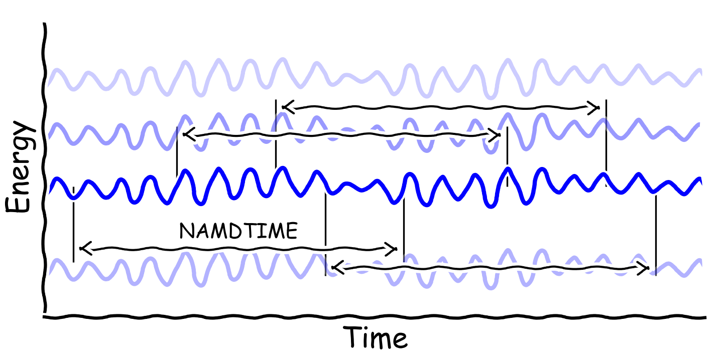
NAMDTIMEis the time for NAMD calculation -
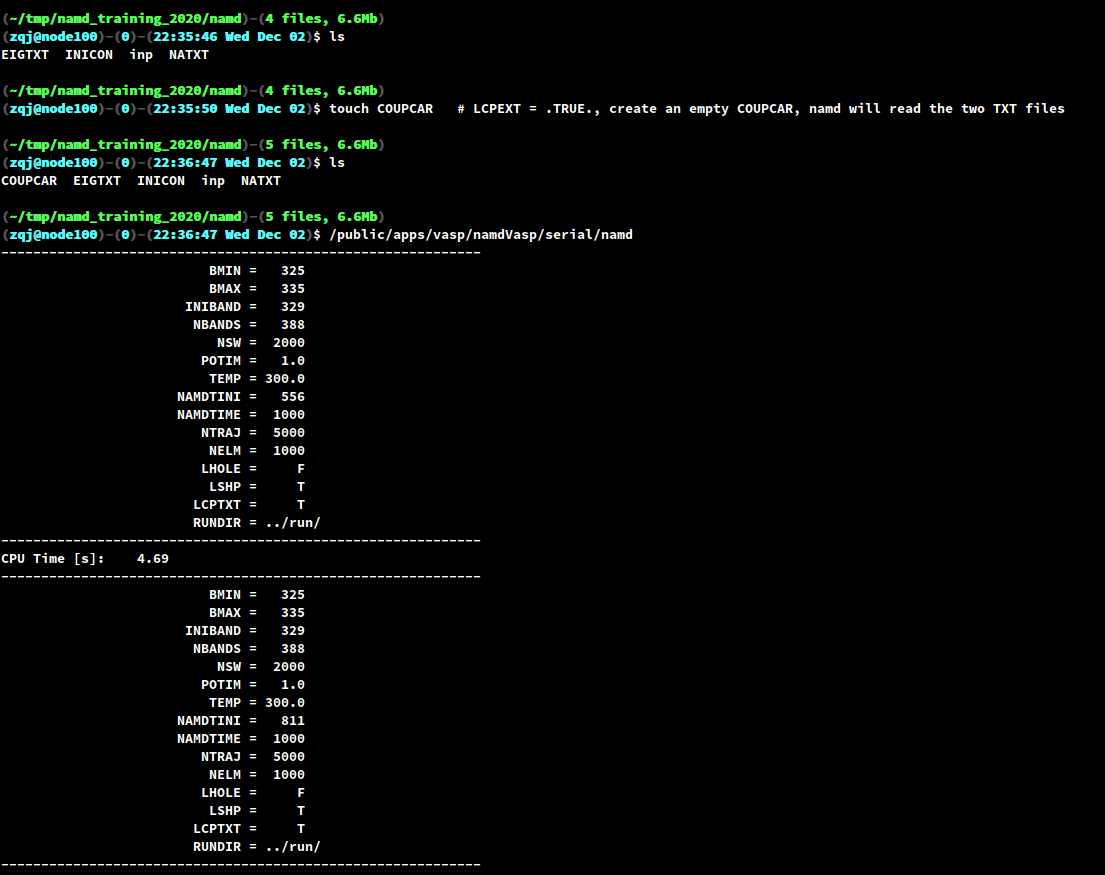
In the first run, the program will check if there exists a file named COUPCAR. If the file does not exist, then the program will read the
WAVECARs and generate theCOUPCAR. TheCOUPCARcontains all the information needed to run an NAMD calculation, i.e. all the nonadiabatic couplings (NAC) and all the Kohn-Sham energies.The
COUPCARis a binary file and is usually very large, about a few gigabytes. Therefore, the program also writes out two text files:EIGTXTandNATXT, which contains the Kohn-Sham energies and NAC contributed by the bands within BMIN and BMAX.If
LCPEXT = .TRUE.and theCOUPCARexist (can be empty), then the program will read the two TXT files and start the NAMD calculation.
Below we show the first few lines of the INICON file.
1
2
3
4
5
6
7
8
9
1 329
2 329
3 329
4 329
5 329
6 329
7 329
8 329
9 329
-
The number of lines in
INICONis given byNSAMPLEininpfile. -
The first column is the initial time. In practice, initial time +
NAMDTIMEshould be less thanNSW, otherwise, there will be segmentation fault. -
The second column is the initial band index of the corresponding initial time. Due to band crossings, the initial band index at different time might be different.
Once the two input files are ready, just type /path/to/your/namd or namd if
you have set the PATH environment variable. In our case, since the COUPCAR
is too large, we will skip the COUPCAR and read the two TXT files.
When the program finishes, you will find two types of output files:
-
PSICT.*files, the suffix of which correspond to the initial time in theINICONfile. Apparently, there areNSAMPLEsuch files. These files contains the time-dependent expansion coefficients. -
SHPROP.*files, with the meaning of the suffix same asPSICT.*. These files contains the populations of the of the selected bands.Utilize this script poen_fssh.py to process
SHPROP.*files and get the time evolution of the populations. The results should look like this:
Below are some customized parameters that that you might want to change:
1
2
3
4
5
6
7
nsw = 2000        # same as NSW of inp
prefix = 'waverpod/run'
                  #
bmin = 324        # python index starts from 0, so this one is the BMIN of inp minus 1
bmax = 335        # the same as BMAX of inp
namdTime = 1000   # same as NAMDTIME of inp
potim = 1.0       # same as POTIM of inp
Contact
-
Dr. Qijing Zheng (郑奇靖), zqj@ustc.edu.cn
-
Mr. Xiang Jiang (蒋翔), jxiang@mail.ustc.edu.cn
-
Dr. Weibin Chu (褚维斌),wbchu@ustc.edu.cn
-
Dr. Chuanyu Zhao (赵传寓),zhaochuanyu@zju.edu.cn
-
Prof. Jin Zhao (赵瑾), zhaojin@ustc.edu.cn