Phonopy: Rutile TiO<sub>2</sub>

Phonon Dispersion of Rutile TiO$_2$

This is a summary of my using Phonopy to calculate phonon spectrum of rutile TiO$_2$. ¹

Computational Details

Below is a list of used packages and computational details

Phonopy
DFT code: VASP version 5.4.4
PAW method, GGA (PBE).
Click here to download the POTCAR I used, where normal Ti POTCAR (4 valence electrons) was used.

Note that if Ti_sv POTCAR (12 valence electrons) is used instead, there will be three imaginary modes at Gamma point, one of which resembles the A_2u mode that is responsible for the incipient ferroelectric behavior in rutile TiO$_2$. To remove the imaginary modes, either DFT+U or LDA should be used.

The lattice constants from different POTCAR and functional:
- PBE + Ti POTCAR:
  
  $a = 4.662\,\mathring{A};\thinspace c=2.969\,\mathring{A}$ and NO imaginary modes at Gamma point.
- PBE + Ti_sv POTCAR:
  
  $a = 4.645\,\mathring{A};\thinspace c=2.967\,\mathring{A}$ and three imaginary moes at Gamma point
- LDA + Ti_sv POTCAR:
  
  $a = 4.554\,\mathring{A};\thinspace c=2.922\,\mathring{A}$ and NO imaginary modes at Gamma point.
ASE for lattice constants optimization.
Matplotlib for plotting. ²

Step by Step Calculation

Optimizing the Lattice Constants

A script utilizing ASE to optimize the lattice constant is used.³ As is shown below, the python script is embedded in the job submission script.

#!/bin/bash
#SBATCH --partition       h3c
#SBATCH --time            12:00:00
#SBATCH --nodes           1
#SBATCH --ntasks-per-node 48
#SBATCH --cpus-per-task   1
#SBATCH --error           out_%j.err
#SBATCH --output          out_%j.log

ulimit -s unlimited

module load vasp/5.4.4
#module load vasp/5.4.4_soc
# module load vasp/6.1.0
#module load vasp/6.1.0_omp

echo "============================================================"
echo "Job ID: $SLURM_JOB_NAME"
echo "Job name: $SLURM_JOB_NAME"
echo "Number of nodes: $SLURM_JOB_NUM_NODES"
echo "Number of processors: $SLURM_NTASKS"
echo "Task is running on the following nodes:"
echo $SLURM_JOB_NODELIST
echo "OMP_NUM_THREADS = $SLURM_CPUS_PER_TASK"
echo "============================================================"
echo
 
python << EOF
import os
import numpy as np
from ase.io import read, write
from ase.calculators.vasp import Vasp
from ase.constraints import UnitCellFilter
from ase.optimize import BFGS as QuasiNewton

os.environ['VASP_COMMAND'] = "srun -n ${SLURM_NPROCS} vasp_std"
os.environ['VASP_PP_PATH'] = "/public/apps/vasp/pp/"

# the starting configuration
geo  = read('init.vasp', format='vasp')
# setting the c-axis parameter
# geo.cell[-1,-1] = 25

calc = Vasp(
        ###############################
        # General
        ###############################
        system = 'vaspCalc',
        prec   = 'Accurate',
        encut  = 500,
        ispin  = 1,
        istart = 0,
        icharg = 1,
        ###############################
        # Electronic relaxation
        ###############################
        # isym   = 0,
        algo   = 'Fast',
        nelmin = 4,
        nelm   = 120,
        xc     = 'pbe',
        ediff  = 1E-8,
        ismear = 0,
        sigma  = 0.04,
        npar   = 4,
        ###############################
        # k-points grid
        ###############################
        kpts   = (15, 15, 23),
        gamma  = True,
        ###############################
        # Writing Flat
        ###############################
        nwrite = 1,
        lwave  = False,
        lcharg = False,
        ###############################
        # Vdw Correction
        ###############################
        # ivdw   = 10,
        ###############################
        # dipole correction
        ###############################
        # ldipol = True,
        # idipol = 3,
        # dipol  = [0.5, 0.5, 0.5]
       )
geo.set_calculator(calc)

# stress mask [XX, YY, ZZ, YZ, XZ, XY]
# 0 if fixed else 1
unf = UnitCellFilter(geo, mask=[1,1,1,1,1,1])
# unf = UnitCellFilter(geo, mask=[1,1,0,0,0,1])
dyn = QuasiNewton(unf, logfile='opt.log', trajectory='opt.traj')

dyn.run(fmax=0.001)

write('final.vasp', geo, vasp5=True, direct=True)
EOF

A few notes

The INCAR, KPOINTS and POTCAR are automatically generated by the script based on the input settings. Therefore, there is NO NEED to prepare these files.
The initial geometry is read from the file init.vasp and POSCAR will be automatically generated by ASE.
Note that the inputs parameters in the script are basically a SCF calculation, i.e. IBRION = -1.
The stopping criteria is in the line dyn.run(fmax=0.001), and the optimized geometry is written in the file final.vasp

Born Effective Charge and Phonon at Gamma-point

As TiO$_2$ is an ionic crystal, there are LO-TO splittings in the optical phonons. One must perform non-analytical (NAC) term correction by calculating Born effective charge.

I used DFPT to get the Born effective charge as well as the phonon at $\Gamma$-point.

General
  SYSTEM = VaspCalc
    PREC = Accurate
   ENCUT = 500 eV
   ISPIN = 1
  ISTART = 1
  ICHARG = 1

Ionic Relaxation
  IBRION = 8

Electronic relaxation
    ALGO = Fast
  NELMIN = 4
    NELM = 100
   EDIFF = 1E-8
  ISMEAR = 0
   SIGMA = 0.04
  LORBIT = 11
   LREAL = .FALSE.
 ADDGRID = .TRUE.

Writing Flag
  NWRITE = 1
   LWAVE = .FALSE.
  LCHARG = .FALSE.
LEPSILON = .TRUE.

Note the last line is the extra setting needed to get Born effective charge.

KPOINTS

When the calculation is finished, used phonopy-vasp-born to get the Born effective charge

phonopy-vasp-born | tee BORN

# epsilon and Z* of atoms 1 3
   7.95986424    0.00000000    0.00000000    0.00000000    7.95986424    0.00000000    0.00000000    0.00000000    9.77308295 
   6.48351229    1.12137427    0.00000000    1.12137427    6.48351229    0.00000000    0.00000000    0.00000000    8.13997738 
  -3.24175614    1.91676778    0.00000000    1.91676778   -3.24175614    0.00000000    0.00000000    0.00000000   -4.06998869 

One can see that there are no negative (imaginary) frequencies, except for three small negative ones which corresponds to translational motion, at the $\Gamma$-point. This means that we have get a fairly optimized cell.

grep THz OUTCAR

f  =   23.488597 THz   147.583210 2PiTHz  783.495252 cm-1    97.141066 meV
f  =   17.390776 THz   109.269470 2PiTHz  580.093838 cm-1    71.922495 meV
f  =   14.411095 THz    90.547583 2PiTHz  480.702388 cm-1    59.599522 meV
f  =   14.411095 THz    90.547583 2PiTHz  480.702388 cm-1    59.599522 meV
f  =   13.186496 THz    82.853200 2PiTHz  439.854157 cm-1    54.534985 meV
f  =   13.186496 THz    82.853200 2PiTHz  439.854157 cm-1    54.534985 meV
f  =   12.217729 THz    76.766257 2PiTHz  407.539569 cm-1    50.528485 meV
f  =   10.984280 THz    69.016267 2PiTHz  366.396131 cm-1    45.427347 meV
f  =   10.667164 THz    67.023770 2PiTHz  355.818290 cm-1    44.115861 meV
f  =   10.667164 THz    67.023770 2PiTHz  355.818290 cm-1    44.115861 meV
f  =    4.322348 THz    27.158111 2PiTHz  144.177992 cm-1    17.875799 meV
f  =    2.690268 THz    16.903451 2PiTHz   89.737671 cm-1    11.126057 meV
f  =    2.690268 THz    16.903451 2PiTHz   89.737671 cm-1    11.126057 meV
f  =    2.592941 THz    16.291927 2PiTHz   86.491191 cm-1    10.723545 meV
f  =    2.393622 THz    15.039568 2PiTHz   79.842622 cm-1     9.899227 meV
f/i=    0.005079 THz     0.031909 2PiTHz    0.169401 cm-1     0.021003 meV
f/i=    0.005079 THz     0.031909 2PiTHz    0.169401 cm-1     0.021003 meV
f/i=    0.005766 THz     0.036231 2PiTHz    0.192342 cm-1     0.023847 meV

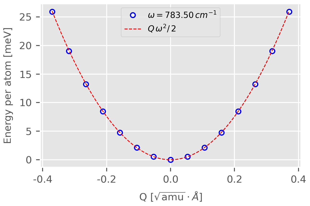
One can show that the Potential Energy Surface (PES) along the normal mode direction is indeed a harmonic potential.

Under the directory which you have performed the Gamma-point phonon calculation, use the script init.sh to initialize and generate a series of displacements along the normal mode (by the script phonon_traj.py).

#!/bin/bash

if [ -f OUTCAR.gz ]; then
    gzip -d OUTCAR.gz
fi

rm -f m_??/traj*.vasp 2>/dev/null

for mode in {01..03}  # select the modes
do
    mkdir -p m_${mode}
    cd m_${mode}
    (( m = mode - 1 ))
    ./phonon_traj.py -i ../OUTCAR -p ../POSCAR -m ${m} -t 300 -msd classical --linear_traj -nsw 15
    for ii in {01..15}
    do
        mkdir -p ${ii}
        cd ${ii}
        ln -sf ../../INCAR_scf INCAR
        ln -sf ../../POTCAR
        ln -sf ../../KPOINTS
        ln -sf ../traj_${ii}.vasp POSCAR
        cd ../
    done
    cd ..
done

gzip OUTCAR

In then script phonon_traj.py, we have set the phonon vibration amplitude according to a classical harmonic oscillator (-msd classical) with termperature 300 Kelvin (-t 300).

Perform SCF calculation in each sub-directories and then plot the result using this script. Below is the result for the first normal mode, from which one can see that the calculated data fit well with the harmonic potential and the maximum PES of $25.8\,\mathrm{meV}$ corresponds well to $T=300\,K$.

**Figure 1.** Potential energy surface along the first normal mode. Blue dots are results from first-principles calculations and red dashed line is the harmonic potential. Figure plotted by Matplotlib.

Phonon Spectrum from Frozen-phonon Method ⁴

Prepare INCAR, KPOINTS, and POSCAR_u, use the script init.sh to initialize the jobs.

 #!/bin/bash
   
 rm POSCAR-* 2>/dev/null
 phonopy -d --dim="3 3 4" -c POSCAR_u
   
 for pos in POSCAR-*
 do
     mkdir -p d_${pos/POSCAR-}
     cd d_${pos/POSCAR-}
     ln -sf ../INCAR
     ln -sf ../POTCAR
     ln -sf ../KPOINTS
     cp ../${pos} POSCAR
     cd ..
 done

The script will create one directory for each displacement POSCAR-00?.

After the calculation in each displacement directory is done, prepare inputs for phonopy to get the phonon band and DOS.

Phonon band: band.conf
1 2 3 DIM = 3 3 4 BAND = AUTO EIGENVECTORS = .TRUE.
Phonon DOS: dos.conf
1 2 3 4 5 DIM = 3 3 4 MP = 51 51 51 DOS = .TRUE. GAMMA_CENTER = .TRUE. FPITCH = 0.02
DO NOT forget to copy the BORN file to current directory to perform NAC term correction.

Use the script pp.sh to create the FORCE_SETS and calculation phonon band and DOS.

#!/bin/bash
if [ ! -f FORCE_SETS ]; then
    phonopy -f d_00?/vasprun.xml
fi
  
phonopy --nac band.conf
phonopy --nac dos.conf
python ph_band-dos.py # One can also use phonopy to plot the result.

In the script pp.sh, a python script ph_band-dos.py is used to plot the band and DOS in one figure, which of course can also be done by phonopy.

The resulting output files:

One can use this site⁵ to visulize the animation of phonon modes by uploading the band.yaml file.

Phonon Band and Density-of-States

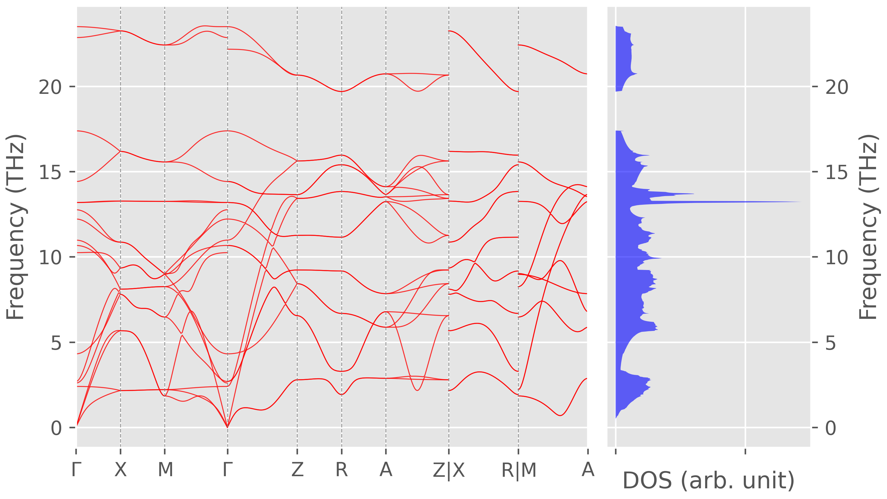
The phonon spectrum of rutile TiO$_2$ with NAC term correction

Figure 2. Phonon dispersion with non-analytical term correction.
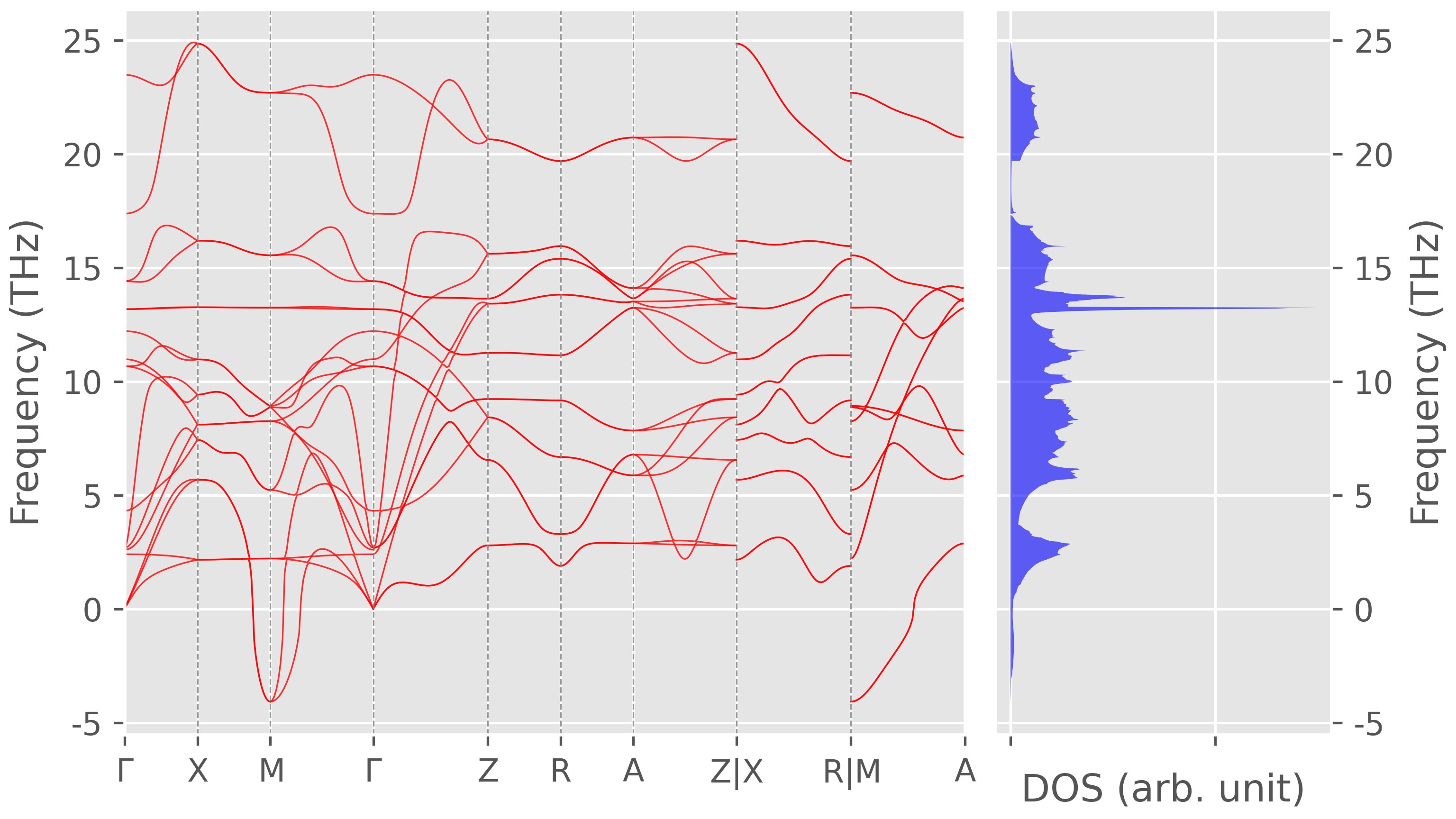
The phonon spectrum of rutile TiO$_2$ without NAC term correction, i.e. remove --nac in the pp.sh.

Figure 3. Phonon dispersion without non-analytical term correction.
One can see that the NAC term correction removes the imaginary frequencies along some $k$-path and generate LO-TO splitting at $\Gamma$ points.
- Due to the NAC term, the phonon frequencies at $\Gamma$ point depend on the direction of $\mathbf{q} \to 0$. As a result, the result of Raman spectra depend on the angle between the incident light and the sample.
- BTW, I thought NAC term correction only affects the phonons near $\Gamma$-point, which seems to be untrue,⁶ as phonopy also perform long-range dipole-dipole correction at general $q$-points.⁷
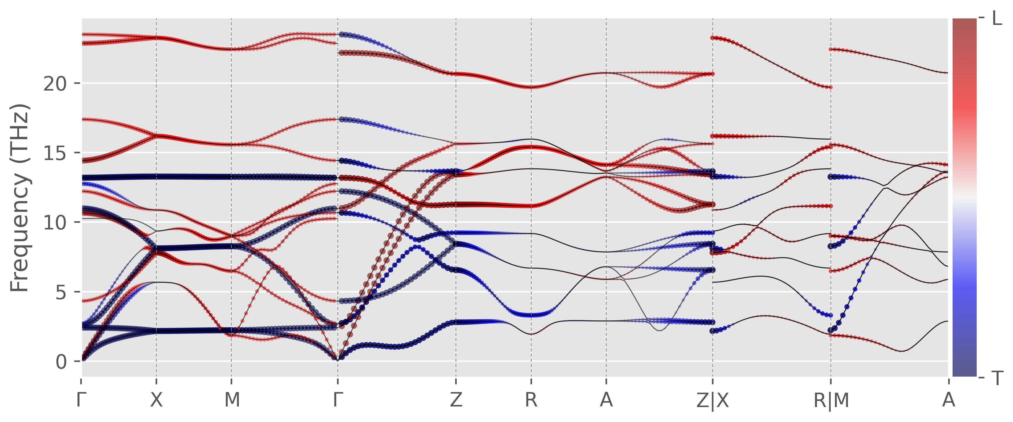
Longitudinal and Tranverse phonon modes

For purely longitudinal phonon mode, the polarization vector of the mode $\mathbf{p}_{nq}$ is parallel to the wavevector $\mathbf{q}$, i.e.
\[\begin{equation*} W_{nk} = \dfrac{\mathbf{p}_{nk}\cdot\mathbf{q}}{|\mathbf{q}|} = 1 \end{equation*}\]
On the other hand, the polarization vector of a purely transverse mode is perpendicular to the wavevector, or
\[\begin{equation*} W_{nk} = \dfrac{\mathbf{p}_{nk}\cdot\mathbf{q}}{|\mathbf{q}|} = 0 \end{equation*}\]
In practice, the classification of purely longitudinal and transverse modes is only valid for isotropic materials. For high symmetry structures (like cubic) and in some high symmetry directions, it is also a very good approximation. But for lower symmetry structures you cannot classify modes as purely transverse or longitudinal. Nevertheless, we can use $W_{nk}$ to quantify the similarness of the mode to longitudinal (close to 1) or transverse modes (close to 0).

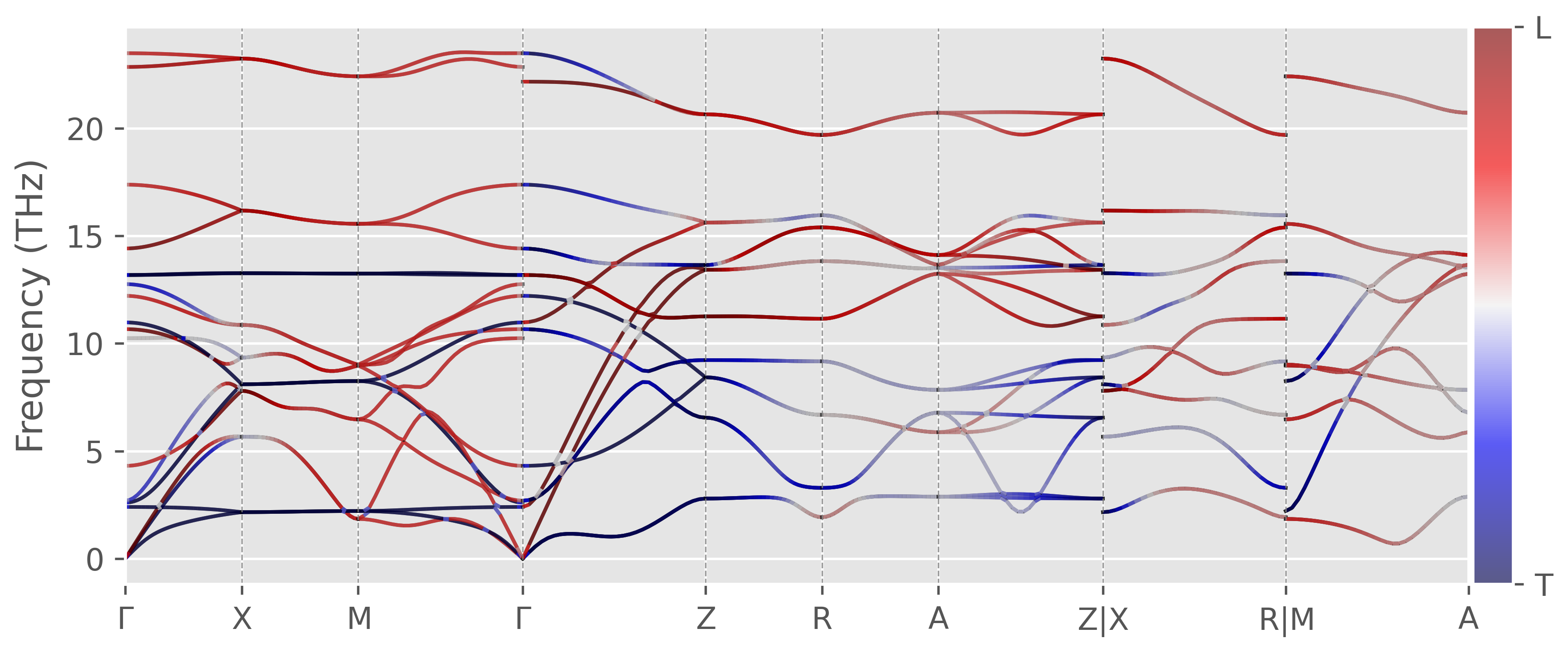
Figure 4. Rutile TiO₂ phonon dispersion overlapped with W_nk, generated by this script.

The same result with color-stripe plot

Figure 5. Rutile TiO₂ phonon dispersion overlapped with W_nk, generated by this script.

References

Material Project: TiO2 ↩
One can of course use the plotting function of Phonopy. ↩
Note that VASP can optimize the lattice constants by setting ISIF=3. ↩
Phonopy & VASP ↩
Phononwebsite ↩
Non-analytical term correction in phonopy ↩
Phonopy: Correction by dipole-dipole interaction ↩

Phonopy: Rutile TiO₂

Phonon Dispersion of Rutile TiO$_2$

Computational Details

Step by Step Calculation

Optimizing the Lattice Constants

Born Effective Charge and Phonon at Gamma-point

Phonon Spectrum from Frozen-phonon Method ⁴

Phonon Band and Density-of-States

References

Trending Tags

Phonopy: Rutile TiO2

Phonon Dispersion of Rutile TiO$_2$

Computational Details

Step by Step Calculation

Optimizing the Lattice Constants

Born Effective Charge and Phonon at Gamma-point

Phonon Spectrum from Frozen-phonon Method 4

Phonon Band and Density-of-States

References

Further Reading

Angular Momentum in Solids

NAC Calculation for 1D Model Hamiltonian

How to Plot the First Brillouin Zone

Trending Tags

Phonopy: Rutile TiO₂

Phonon Spectrum from Frozen-phonon Method ⁴