
Introduction
The translational symmetry of solids resulits in a quantum number, i.e. the crystal momentum $\mathbf{k}$. Consequently many quantities of the crystal, e.g. total energy and density of states, require integration over the Brillouin Zone (BZ). The integrations are generally of the form
\[\begin{equation} \label{eq:bz_int} \frac{1}{\Omega_{BZ}}\int_{BZ} \,M_{\mathbf{k}}\cdot f(\varepsilon_\mathbf{k})\,\mathrm{d}\mathbf{k} \end{equation}\]where $M_{\mathbf{k}}$ is the matrix element and $f(\varepsilon_\mathbf{k})$ is Heaviside step function $\Theta(E - \varepsilon_\mathbf{k})$ or Dirac function $\delta(E - \varepsilon_\mathbf{k})$.
There are generally two categories of methods to perform the integration: the special-point method and the tetrahedron method, where the former method is often combined with smearing method to improve convergence.1 The most widely used sets of special points are those of Monkhorst and Pack,2 however, it is beyond the scope of the current post to discuss it.
Tetrahedron Method
- In the tetrahedron method, the reciprocal space is first divided into small sub-meshes, which are then further divided into tetrahedra, as is shown in Figure 1.
- Within each tetrahedron, the quantity $M_{\mathbf{k}}$ and $\varepsilon_\mathbf{k}$ are linearly or quadraticly interpolated and as a result, the BZ integration can be done analytically. We will focus on the linear interpolation case, known as linear tetrahedron method.3
Linear Tetrahedron method
In the linear tetrahedron method, the quantities, $M_\mathrm{k}$ and $\varepsilon_\mathbf{k}$, are linearly interpolated within the tetrahedron, i.e.
\[\begin{equation} \varepsilon(x, y, z) = a + b\cdot x + c\cdot y + d\cdot z \end{equation}\]where $x, y, z$ are the three component of $\mathbf{k}$. With the values at the four vertices, e.g. $\varepsilon_i (i=1,4)$, the coeffiecients $a$, $b$, $c$ and $d$ can be readily obtained. One can also use the Barycentric coordinates4 of the tetrahedron and express the quantity as
\[\begin{equation} \label{eq:barycentric_exp} \varepsilon(e, u, v) = \varepsilon_1\cdot(1 - e - u - v) + \varepsilon_2 \cdot e + \varepsilon_3 \cdot u + \varepsilon_4 \cdot v \end{equation}\]where
\[\begin{align} x &= x_1\cdot(1 - e - u - v) + x_2 \cdot e + x_3 \cdot u + x_4 \cdot v \\ y &= y_1\cdot(1 - e - u - v) + y_2 \cdot e + y_3 \cdot u + y_4 \cdot v \\ z &= z_1\cdot(1 - e - u - v) + z_2 \cdot e + z_3 \cdot u + z_4 \cdot v \\ \end{align}\]and $e, u, v \in [0, 1]$.
Now the contribution within the tetrahedron to the BZ integration becomes
\[\begin{equation} \frac{1}{\Omega_{BZ}}\int_{BZ}\, M(e, u, v) \cdot f(\varepsilon(e, u, v)) \cdot \frac{\partial(x, y, z)}{\partial(e, u, v)} \, \mathrm{d}e \mathrm{d}u \mathrm{d}v \end{equation}\]where $\frac{\partial(x, y, z)}{\partial(e, u, v)}$ is the Jacobi determinant and one can readily show that it equals to $6\Omega_T$ where $\Omega_T$ is the volume of the tetrahedron.5
Density of States (DOS)
For the density of state (DOS), the quantity $M_\mathbf{k} =1$ and $f(\varepsilon_\mathbf{k})$ is the Dirac function. In this case, the contribution of the i-th tetrahedron $T_i$ to the DOS is
\[\begin{align} \label{eq:dos} \rho(E) &= \frac{1}{\Omega_{BZ}}\int_{T_i}\, \delta(E - \varepsilon(e, u, v)) \cdot \frac{\partial(x, y, z)}{\partial(e, u, v)} \, \mathrm{d}e \mathrm{d}u \mathrm{d}v \\[9pt] &= \frac{6\Omega_T}{\Omega_{BZ}}\int_{T_i}\, \frac{1}{|\nabla \varepsilon(e, u, v)|} \, \mathrm{d}S\Bigr|_{\varepsilon = E} \end{align}\]where the volume integration over the BZ becomes a surface integration on an iso-value plane. Moreover, let us assumed $\varepsilon_i$ is ordered according to increasing values, i.e. $\varepsilon_1 < \varepsilon_2 < \varepsilon_3 < \varepsilon_4$ and denote $\varepsilon_{ji} = \varepsilon_j - \varepsilon_i$, where $\varepsilon_0 = E$.
The norm of the derivative can be reaily get from Eq.\eqref{eq:barycentric_exp}
\[\begin{equation} |\nabla\varepsilon(e, u, v)| = \sqrt{\varepsilon_{21}^2+\varepsilon_{31}^2+\varepsilon_{41}^2} \end{equation}\]For different value of the energy $E$, the iso-value surfaces intersected with the tetrahedron are differnt:
-
For $\varepsilon_4 < E$ or $E > \varepsilon_E$
No intersection between the iso-surface and the tetrahedron, hence no contribution to DOS within this tetrahedron.
-
For $\varepsilon_1 < E < \varepsilon_2$
The iso-surface is a triangle, as is shown in Figure 2. The coordinates of vertices of the triangle $\vec{c_i}$ can be readily obtained from Eq.\eqref{eq:barycentric_exp}
\[\begin{align} \vec{c_1} \quad&\Rightarrow\quad \begin{pmatrix} \dfrac{\varepsilon_{01}}{\varepsilon_{21}}, & 0, & 0 \end{pmatrix} \\[9pt] \vec{c_2} \quad&\Rightarrow\quad \begin{pmatrix} 0, & \dfrac{\varepsilon_{01}}{\varepsilon_{31}}, & 0 \end{pmatrix} \\[9pt] \vec{c_3} \quad&\Rightarrow\quad \begin{pmatrix} 0, & 0, & \dfrac{\varepsilon_{01}}{\varepsilon_{41}} \end{pmatrix} \\[9pt] \end{align}\]The area of the iso-surface is then given by
\[\begin{equation} \frac{1}{2}\cdot|(\vec{c_1} - \vec{c_3})\times(\vec{c_2} - \vec{c_3})| = \frac{1}{2} \cdot \varepsilon_{01}^2 \cdot \frac{\sqrt{\varepsilon_{21}^2+\varepsilon_{31}^2+\varepsilon_{41}^2}} {\varepsilon_{21}\varepsilon_{31}\varepsilon_{41}} \end{equation}\]1 2 3 4 5 6 7 8 9 10 11 12 13 14 15 16 17 18
#!/usr/bin/env python # -*- coding: utf-8 -*- import sympy as sp e01, e21, e31, e41 = sp.symbols('e01, e21, e31, e41') c1 = sp.Matrix([e01/e21, 0, 0]) c2 = sp.Matrix([0, e01/e31, 0]) c3 = sp.Matrix([0, 0, e01/e41]) s1 = (c1 - c3).cross(c2 - c3) sp.pprint(sp.simplify(sp.sqrt(s1.dot(s1)))) # ___________________________ # ╱ 4 ⎛ 2 2 2⎞ # ╱ e₀₁ ⋅⎝e₂₁ + e₃₁ + e₄₁ ⎠ # ╱ ───────────────────────── # ╱ 2 2 2 # ╲╱ e₂₁ ⋅e₃₁ ⋅e₄₁ #
Therefore, the contribution to the DOS is
\[\begin{equation} \rho_1(E) = \frac{\Omega_T}{\Omega_{BZ}} \cdot \frac{3\cdot \varepsilon_{01}^2} {\varepsilon_{21}\varepsilon_{31}\varepsilon_{41}} \end{equation}\] -
For $\varepsilon_2 < E < \varepsilon_3$
The iso-surface is a tetragon, as is shown in Figure 2. Again, the coordinates of vertices of the tetragon are given by
\[\begin{align} \vec{c_1} \quad&\Rightarrow\quad \begin{pmatrix} \dfrac{\varepsilon_{40}}{\varepsilon_{42}}, & 0, & -\dfrac{\varepsilon_{20}}{\varepsilon_{42}} \end{pmatrix} \\[9pt] \vec{c_2} \quad&\Rightarrow\quad \begin{pmatrix} \dfrac{\varepsilon_{30}}{\varepsilon_{32}},& -\dfrac{\varepsilon_{20}}{\varepsilon_{32}},& 0 \end{pmatrix} \\[9pt] \vec{c_3} \quad&\Rightarrow\quad \begin{pmatrix} 0,& \dfrac{\varepsilon_{01}}{\varepsilon_{31}},& 0 \end{pmatrix} \\[9pt] \vec{c_4} \quad&\Rightarrow\quad \begin{pmatrix} 0,& 0,& \dfrac{\varepsilon_{01}}{\varepsilon_{41}} \end{pmatrix} \\[9pt] \end{align}\]The area of the iso-surface is then given by
\[\begin{align*} S &= \frac{1}{2}\cdot \Bigl| \left[ (\vec{c_1} - \vec{c_4}) + (\vec{c_2} - \vec{c_4}) \right] \times(\vec{c_2} - \vec{c_4}) \Bigr| \\[9pt] &= \frac{1}{2} \cdot \frac{\sqrt{\varepsilon_{21}^2+\varepsilon_{31}^2+\varepsilon_{41}^2}} {\varepsilon_{31}\varepsilon_{41}} \cdot \left[ \varepsilon_{21} - 2\varepsilon_{20} - \frac{\varepsilon_{20}^2\cdot(\varepsilon_{31} + \varepsilon_{42})} {\varepsilon_{32}\varepsilon_{42}} \right] \end{align*}\]1 2 3 4 5 6 7 8 9 10 11 12 13 14 15 16 17 18 19 20 21 22 23 24 25 26 27 28 29 30 31 32 33 34 35 36 37 38 39 40 41 42 43 44 45 46 47 48 49 50
#!/usr/bin/env python # -*- coding: utf-8 -*- import sympy as sp e43, e42, e41, e40, e32, e31, e30, e21, e20, e10 = sp.symbols( 'e43, e42, e41, e40, e32, e31, e30, e21, e20, e10' ) c1 = sp.Matrix([e40 / e42, 0, - e20 / e42]) c2 = sp.Matrix([e30 / e32, -e20 / e32, 0]) c3 = sp.Matrix([0, -e10 / e31, 0]) c4 = sp.Matrix([0, 0, -e10 / e41]) s1 = (c1 + c3 - 2 * c4).cross(c2 - c4) sp.pprint( sp.simplify( sp.sqrt(s1.dot(s1)) ) ) # _______________________________________________________________________________________________________________________________________ # ╱ 2 # ╱ 2 2 2 2 ⎛ 2 ⎞ # ╱ e₃₁ ⋅(e₁₀⋅e₃₂⋅e₄₀ - e₃₀⋅(2⋅e₁₀⋅e₄₂ - e₂₀⋅e₄₁)) + e₄₁ ⋅(e₁₀⋅e₃₀⋅e₄₂ - e₂₀⋅e₃₁⋅e₄₀) + ⎝e₁₀ ⋅e₃₂⋅e₄₂ - e₂₀⋅e₃₁⋅(2⋅e₁₀⋅e₄₂ - e₂₀⋅e₄₁)⎠ # ╱ ───────────────────────────────────────────────────────────────────────────────────────────────────────────────────────────────────── # ╱ 2 2 2 2 # ╲╱ e₃₁ ⋅e₃₂ ⋅e₄₁ ⋅e₄₂ # one can show that the expression within the braces are identical, i.e. # 2 2 # (e₁₀⋅e₃₂⋅e₄₀ - e₃₀⋅(2⋅e₁₀⋅e₄₂ - e₂₀⋅e₄₁)) = (e₁₀⋅e₃₀⋅e₄₂ - e₂₀⋅e₃₁⋅e₄₀) # 2 # ⎛ 2 ⎞ 2 2 # ⎝e₁₀ ⋅e₃₂⋅e₄₂ - e₂₀⋅e₃₁⋅(2⋅e₁₀⋅e₄₂ - e₂₀⋅e₄₁)⎠ = e₂₁ ⋅(e₀₁⋅e₃₀⋅e₄₂ + e₂₀⋅e₃₁⋅e₄₀) # sp.pprint( sp.expand( (e42*(e32 + e20)*(e21 - e20) - e20*e31*(e42 + e20)) ) ) # 0 < (e₀₁⋅e₃₀⋅e₄₂ + e₂₀⋅e₃₁⋅e₄₀) = # # 2 2 # - e₂₀ ⋅e₃₁ - e₂₀ ⋅e₄₂ + e₂₀⋅e₂₁⋅e₄₂ - e₂₀⋅e₃₁⋅e₄₂ - e₂₀⋅e₃₂⋅e₄₂ + e₂₁⋅e₃₂⋅e₄₂ = # # 2 # - e₂₀ ⋅(e₃₁ + e₄₂) - 2⋅e₂₀⋅e₃₂⋅e₄₂ + e₂₁⋅e₃₂⋅e₄₂
Therefore, the contribution to the DOS is
\[\begin{equation} \rho_2(E) = \frac{\Omega_T}{\Omega_{BZ}} \cdot \frac{1}{\varepsilon_{31}\varepsilon_{41}} \cdot \left[ 3\varepsilon_{21} - 6\varepsilon_{20} - 3\frac{\varepsilon_{20}^2\cdot(\varepsilon_{31} + \varepsilon_{42})} {\varepsilon_{32}\varepsilon_{42}} \right] \end{equation}\] -
For $\varepsilon_3 < E < \varepsilon_4$
The iso-surface is a triangle, as is shown in Figure 2. The coordinates of vertices of the triangle $\vec{c_i}$
\[\begin{align} \vec{c_1} \quad&\Rightarrow\quad \begin{pmatrix} \dfrac{\varepsilon_{40}}{\varepsilon_{42}}, & 0, & -\dfrac{\varepsilon_{20}}{\varepsilon_{42}} \end{pmatrix} \\[9pt] \vec{c_2} \quad&\Rightarrow\quad \begin{pmatrix} 0, & \dfrac{\varepsilon_{40}}{\varepsilon_{43}}, & -\dfrac{\varepsilon_{30}}{\varepsilon_{43}} \end{pmatrix} \\[9pt] \vec{c_3} \quad&\Rightarrow\quad \begin{pmatrix} 0, & 0, & \dfrac{\varepsilon_{01}}{\varepsilon_{41}} \end{pmatrix} \\[9pt] \end{align}\]The area of the iso-surface is then given by
\[\begin{equation} \frac{1}{2}\cdot|(\vec{c_1} - \vec{c_3})\times(\vec{c_2} - \vec{c_3})| = \frac{1}{2} \cdot \varepsilon_{40}^2 \cdot \frac{\sqrt{\varepsilon_{21}^2+\varepsilon_{31}^2+\varepsilon_{41}^2}} {\varepsilon_{41}\varepsilon_{42}\varepsilon_{43}} \end{equation}\]1 2 3 4 5 6 7 8 9 10 11 12 13 14 15 16 17 18 19 20 21 22 23 24 25 26 27
#!/usr/bin/env python # -*- coding: utf-8 -*- import sympy as sp e43, e42, e41, e40, e30, e20, e10 = sp.symbols( 'e43, e42, e41, e40, e30, e20, e10' ) c1 = sp.Matrix([e40 / e42, 0, - e20 / e42]) c2 = sp.Matrix([0, e40 / e43, - e30 / e43]) c3 = sp.Matrix([0, 0, -e10 / e41]) s1 = (c1 - c3).cross(c2 - c3) sp.pprint(sp.simplify(sp.sqrt(s1.dot(s1)))) # ________________________________________________________________ # ╱ 2 ⎛ 2 2 2 2⎞ # ╱ e₄₀ ⋅⎝e₄₀ ⋅e₄₁ + (e₁₀⋅e₄₂ - e₂₀⋅e₄₁) + (e₁₀⋅e₄₃ - e₃₀⋅e₄₁) ⎠ # ╱ ────────────────────────────────────────────────────────────── # ╱ 2 2 2 # ╲╱ e₄₁ ⋅e₄₂ ⋅e₄₃ # one can easily show that # (e₁₀⋅e₄₂ - e₂₀⋅e₄₁) = -e₄₀⋅e₂₁ # and # (e₁₀⋅e₄₃ - e₃₀⋅e₄₁) = -e₄₀⋅e₃₁
Therefore, the contribution to the DOS is
\[\begin{equation} \rho_3(E) = \frac{\Omega_T}{\Omega_{BZ}} \cdot \frac{3\cdot\varepsilon_{40}^2} {\varepsilon_{41}\varepsilon_{42}\varepsilon_{43}} \end{equation}\]
No. of States
The number of states $n(E)$ is simply the integration of the DOS, i.e.
\[\begin{equation} n(E) = \int_0^E \rho(E)\, \mathrm{d}E \end{equation}\]As a result, the contributions of the i-th tetrahedron to the no. of states are
- For $E < \varepsilon_1$
- For $\varepsilon_1 < E \le \varepsilon_2$
- For $\varepsilon_2 < E \le \varepsilon_3$
- For $\varepsilon_3 < E \le \varepsilon_4$
- For $\varepsilon_4 < E$
$M_\mathbf{k} \ne 1$
For the case of of general $M_\mathbf{k}$, please refer to the paper by A.H. MacDonald et al., 6 where the deduction was started from $f(\varepsilon_\mathbf{k})$ being a step function and the Dirac delta function case is simply the energy derivative of the former.
DOS: Smearing vs. Linear-tetrahedron Method
For the calculation of DOS, another often used method is the so-called smearing method, i.e. use a broadening function, for example Gaussian or Lorentzian shape function, to mimic the Dirac function.
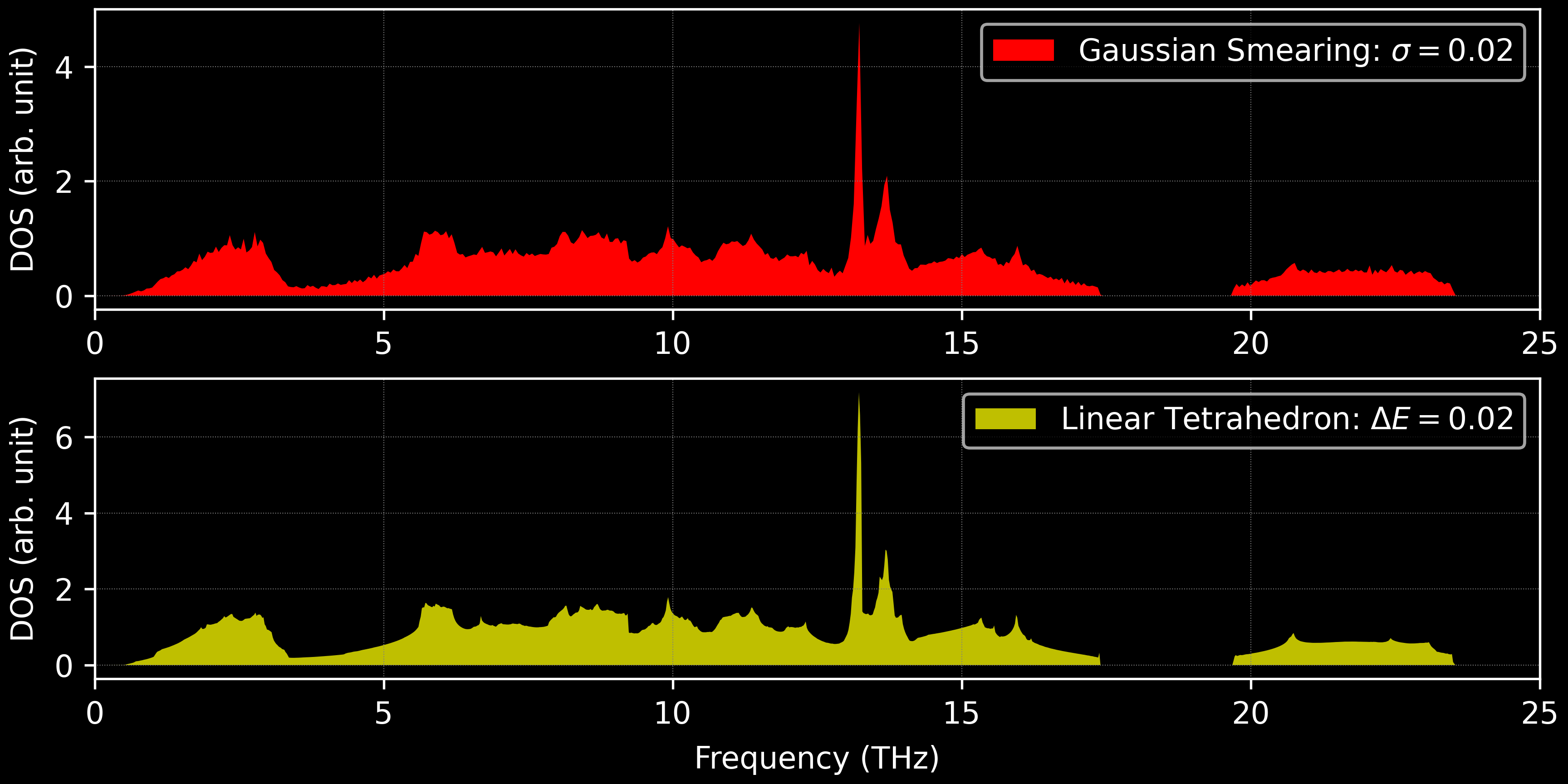
As can be seen from Figure 3, with the same density of BZ sampling, the DOS plot from linear-tetrahedron method is much smoother.
Code Examples
References
-
“High-precision sampling for Brillouin-zone integration in metals”, M. Methfessel and A. T. Paxton, Phys. Rev. B, 40, 3616 (1989) ↩
-
“Special points for Brillouin-zone integrations”, HL Monkhorst et al., Phys. Rev. B, 13, 5188 (1976) ↩
-
“Improved Tetrahedron Method for Brillouin-Zone Integrations”, Peter E. Blöchl et al., Phys. Rev. B, 49, 16223 (1994) ↩
-
Extensions of the tetrahedron method for evaluating spectral properties of solids ↩
-
“Improved tetrahedron method for the Brillouin-zone integration applicable to response functions”, Phys. Rev. B, 89, 094515 (2014) ↩