Time-dependent Schrödinger Equation
The single-particle time-dependent Schrödinger equation of an electron under an external potential read
\[\begin{align} i\hbar \frac{\partial}{\partial t} \psi(\mathbf{r}, t) &= {\cal H}(\mathbf{r};t)\,\psi(\mathbf{r}, t) = [\hat{T} + \hat{V}]\,\psi(\mathbf{r}, t) \\ &=\left[ -\frac{\hbar^2}{2m}\nabla^2 + \hat{V}(\mathbf{r}) \right]\psi(\mathbf{r}, t) \end{align}\]In the atomic unit ($\hbar = m_e = e = a_0 = 1$), 1 the equation becomes
\[\begin{equation} i \frac{\partial}{\partial t} \psi(\mathbf{r}, t) = \left[ -\frac{1}{2}\nabla^2 + \hat{V}(\mathbf{r}) \right]\psi(\mathbf{r}, t) \end{equation}\]The formal solution to the Schrödinger equation
\[\begin{equation} \psi(\mathbf{r}, t+\Delta t) = e^{-i{\cal H}\cdot \Delta t}\,\psi(\mathbf{r}, t) = {\cal U}(\Delta t)\,\psi(\mathbf{r}, t) \end{equation}\]Note that ${\cal U}(t)$ is a unitary operator, which means that the norm of wavefunction is conserved during the time propagation. Therefore, we can use the norm of the wavefunction as an indicator of the time evolution.
If, for example, ${\cal H}$ is time-independent and $\phi_k(\mathbf{r})$ are the corresponding eigenfunctions with eigenvalue $\varepsilon_k$, then one can expand the time-dependent wavefunctions $\psi_j(\mathbf{r}, t)$ by $\phi_k$, i.e.
\[\begin{equation} \psi_j(\mathbf{r}, t) = \sum_k c_k(t)\phi_k(\mathbf{r}) \end{equation}\]As a result, we have
\[\begin{equation} \psi_j(\mathbf{r}, t) = e^{-i{\cal H}\cdot t}\,\psi_j(\mathbf{r}, 0) = \sum_k e^{-i\varepsilon_k t}\,c_k(0)\phi_k(\mathbf{r}) \end{equation}\]Crank-Nicolson Method
The Crank-Nicolson method2 is a combination of forward-Euler method and backward-Euler method.
-
Fowrard-Euler Method
\[\begin{equation} \label{eq:f_euler} \psi_j^{n+1} = e^{-i{\cal H}\Delta t}\cdot \psi_j^n \approx (1 - i{\cal H}\Delta t)\cdot \psi_j^n \end{equation}\] -
Backward-Euler Method
\[\begin{equation} \label{eq:b_euler} e^{i{\cal H}\Delta t}\cdot \psi_j^{n+1}=\psi_j^n \quad\Rightarrow\quad (1 + i{\cal H}\Delta t)\cdot \psi_j^{n+1} \approx \psi_j^n \end{equation}\] -
Crank-Nicolson Method
\[\begin{align} \psi_j^{n+1} = \dfrac{ e^{-i{\cal H}\Delta t/2} }{ e^{i{\cal H}\Delta t/2} }\cdot \psi_j^n &\approx \dfrac{ (1 - i{\cal H}\Delta t/2) }{ (1 + i{\cal H}\Delta t/2) }\cdot \psi_j^n \\[9pt] {\cal U}(\Delta t) & =\dfrac{ (1 - i{\cal H}\Delta t/2) }{ (1 + i{\cal H}\Delta t/2) } \label{eq:cn_cayley_form} \end{align}\]The approximation form to the unitary operator in Eq.\eqref{eq:cn_cayley_form} is also known as Cayley’s form. We can also write the above equation as
\[\begin{equation} \label{eq:cn_form2} (1 + i{\cal H}\Delta t/2)\cdot \psi_j^{n+1} \approx (1 - i{\cal H}\Delta t/2)\cdot \psi_j^n \end{equation}\]Apparently, the equation above can also be obtained by combining Eq.\eqref{eq:f_euler} and \eqref{eq:b_euler}. Note, however, that the method itself is not simply the average of those two methods, as the backward-Euler equation has an implicit dependence on the solution. Moreover, the Crank-Nicolson method is a unitary method, which conserves the norm of the wavefunction, as opposed to the forward- and backward-Euler methods.
Discretization of the Wavefunction
-
In order to solve the equation numerically, let’s first discretize the wavefunction in space and time, equally spaced by $\Delta r$ and $\Delta t$, respectively. Then, denote the wavefunction at $\mathbf{r}_j$ and $t_n = n \cdot \Delta t + t_0$ as $\psi_j^n$. Note that $j$ here is a compound index representing the index of the space grid, e.g. $(j, k, l)$ in 3D case.
-
The time derivative
\[\begin{equation} \frac{\partial\psi(\mathbf{r}_j, t^n)}{\partial t} \approx \frac{\psi_j^{n+1} - \psi_j^n}{\Delta t} \end{equation}\] -
The spatial derivative 3
\[\begin{equation} \label{eq:spatial_deriv} \nabla^2 \psi(\mathbf{r}_j, t^n) \approx \frac{\psi_{j+1}^n + \psi_{j-1}^n- 2\cdot\psi_j^n}{(\Delta r)^2} \end{equation}\]Note that the index $j$ should be considered as a compound index. For example, in a 2-dimensional grid, the space derivative in the $x/y$ directions
\[\begin{align} \nabla_x^2 \psi(\mathbf{r}_{j,k}, t^n) &\approx \frac{\psi_{j+1,k}^n + \psi_{j-1,k}^n- 2\cdot\psi_{j,k}^n}{(\Delta x)^2} \\ \nabla_y^2 \psi(\mathbf{r}_{j,k}, t^n) &\approx \frac{\psi_{j,k+1}^n + \psi_{j,k-1}^n- 2\cdot\psi_{j,k}^n}{(\Delta y)^2} \end{align}\]
1D Schrödinger Equation
Suppose the potential/wavefunction is defined on a set of $J + 1$ spatial grids points $x_j = x_0 + j \Delta x$, with $j \in [0, J]$ and $x_0$ representing the left boundary.
-
Let’s represent the wavefunction at time $t^n$ and $t^{n+1}$ as column vectors, i.e.
\[\begin{align} \Psi^n &= \begin{bmatrix} \psi_0^n& \psi_1^n& \psi_2^n& \cdots& \psi_J^n \end{bmatrix}^T \\[6pt] \Psi^{n+1} &= \begin{bmatrix} \psi_0^{n+1}& \psi_1^{n+1}& \psi_2^{n+1}& \cdots& \psi_J^{n+1} \end{bmatrix}^T \end{align}\] -
From Eq.\eqref{eq:spatial_deriv}, one can readily see that the kinetic operator $\hat{T}$ can be represented by a tri-diagonal matrix of order $J+1$, i.e.
\[\begin{equation} T = -\dfrac{1}{2}\nabla^2 = -\dfrac{1}{2\Delta x^2} \cdot \begin{bmatrix} -2& 1& 0& 0& \ldots& 0& 0& 0 \\ 1& -2& 1& 0& \ldots& 0& 0& 0 \\ 0& 1& -2& 1& \ldots& 0& 0& 0 \\ \vdots& \vdots& \vdots& \vdots& \vdots& \vdots& \vdots& \vdots \\ 0& 0& 0& 0& \ldots& 1& -2& 1 \\ 0& 0& 0& 0& \ldots& 0& 1& -2 \\ \end{bmatrix} \end{equation}\]Note that by writing in this form, we are implicitly assuming zero-boundary condition, i.e. $\psi(x_0, t^n) = 0$ and $\psi(x_J, t^n) = 0$. Or in other words, the values of the potential at the boundaries are infinite.
-
The potential operator $\hat{V}$, on the other hand, is a diagonal matrix.
\[\begin{equation} V = \mathrm{Diag} \begin{bmatrix} v_0& v_1& v_2& \cdots& v_J \end{bmatrix} \end{equation}\] -
The Crank-Nicolson method in Eq.\eqref{eq:cn_form2} in matrix form can then be obtained
\[\begin{align} \label{eq:cn_mat_form} U_2\cdot \Psi^{n+1} &= U_1\cdot \Psi^n \\[9pt] U_2 &= \mathbb{I} + \dfrac{i\Delta t}{2}\cdot [T + V] \label{eq:cn_mat_u2} \\[6pt] U_1 &= \mathbb{I} - \dfrac{i\Delta t}{2}\cdot [T + V] \label{eq:cn_mat_u1} \end{align}\]where $\mathbb{I}$ in Eq.\eqref{eq:cn_mat_u2} and \eqref{eq:cn_mat_u1} is an indentity matrix of order $J+1$. Eq.\eqref{eq:cn_mat_form} is of the form of a linear equation $A\cdot x = b$, which can be solved by using, for example
scipy.sparse.linalg.spsolvein python, given that $U_2$ and $U_1$ are sparse matrices. An example code using python can be found below.1 2 3 4 5 6 7 8 9 10 11 12
# JxN array to store all the wavefunctions PSI = np.zeros((J, N), dtype=complex) # initial wavefunction PSI[:,0] = psi0 # LU decomposition of U2 LU = scipy.sparse.linalg.splu(U2) # Crank-Nicolson evolution for tt in range(0, N-1): # U1 apply on wavefunction at t^n b = U1.dot(PSI[:,tt]) # wavefunction at next step PSI[:,tt+1] = LU.solve(b)
1D Gaussian Wavepacket in an Infinite-well Potential
Let’s first look at the case for $V(x) = 0$, where $x\in[-L/2, L/2]$. As we have stated above, this does not mean that the wavefunction propagates in a free space. Rather, it is a infinitly deep well, since we are adopting a zero-boundary condition.
The initial wavefunction is chosen to be a Gaussian wavepacket4 centered at $x_0$ and with average momentum $k_0$, which is given by
\[\begin{equation} \psi_0(x) = \dfrac{1}{\sqrt[4]{\pi\sigma_x^2}} \cdot e^{i\cdot k_0(x - x_0)} \cdot e^{-\frac{(x - x_0)^2}{2\sigma_x^2}} \end{equation}\]The python codes are shown below.
1
2
3
4
5
6
7
8
9
10
11
12
13
14
15
16
17
18
19
20
21
22
23
24
25
26
27
28
29
30
31
32
33
34
35
36
37
38
39
40
41
42
43
44
45
46
47
48
49
50
  #!/usr/bin/env python

  import numpy as np
  import scipy.sparse as spa
  from scipy.sparse.linalg import splu
  ################################################################################

  def gaussian_wavepacket(x, x0, k, sigma=0.1):
      '''
      One dimensional Gaussian wavepacket
      '''

      x = np.asarray(x)
      g = np.sqrt(1 / np.sqrt(np.pi) / sigma) * np.exp(-(x - x0)**2 / 2 / sigma**2)

      return np.exp(1j * k*(x-x0)) * g

  def CrankNicolson(psi0, V, x, dt, N=100, print_norm=False):
      '''
      Crank-Nicolson method for the 1D Schrodinger equation.
      '''
      # No. of spatial grid points
      J  = x.size - 1
      dx = x[1] - x[0]

      # the external potential
      V = spa.diags(V)
      # the kinetic operator
      O = np.ones(J+1)
      T = (-1 / 2 / dx**2) * spa.spdiags([O, -2*O, O], [-1, 0, 1], J+1, J+1)

      # the two unitary matrices
      U2 = spa.eye(J+1) + (1j * 0.5 * dt) * (T + V)
      U1 = spa.eye(J+1) - (1j * 0.5 * dt) * (T + V)
      # splu requires CSC matrix format for efficient decomposition
      U2 = U2.tocsc()
      LU = splu(U2)

      # Store all the wavefunctions
      PSI_t = np.zeros((J+1, N), dtype=complex)
      # the initial wavefunction
      PSI_t[:, 0] = psi0

      for n in range(N-1):
          b            = U1.dot(PSI_t[:,n])
          PSI_t[:,n+1] = LU.solve(b)
          if print_norm:
              print(n, np.trapz(np.abs(PSI_t[:,n+1])**2, x))

      return PSI_t
-
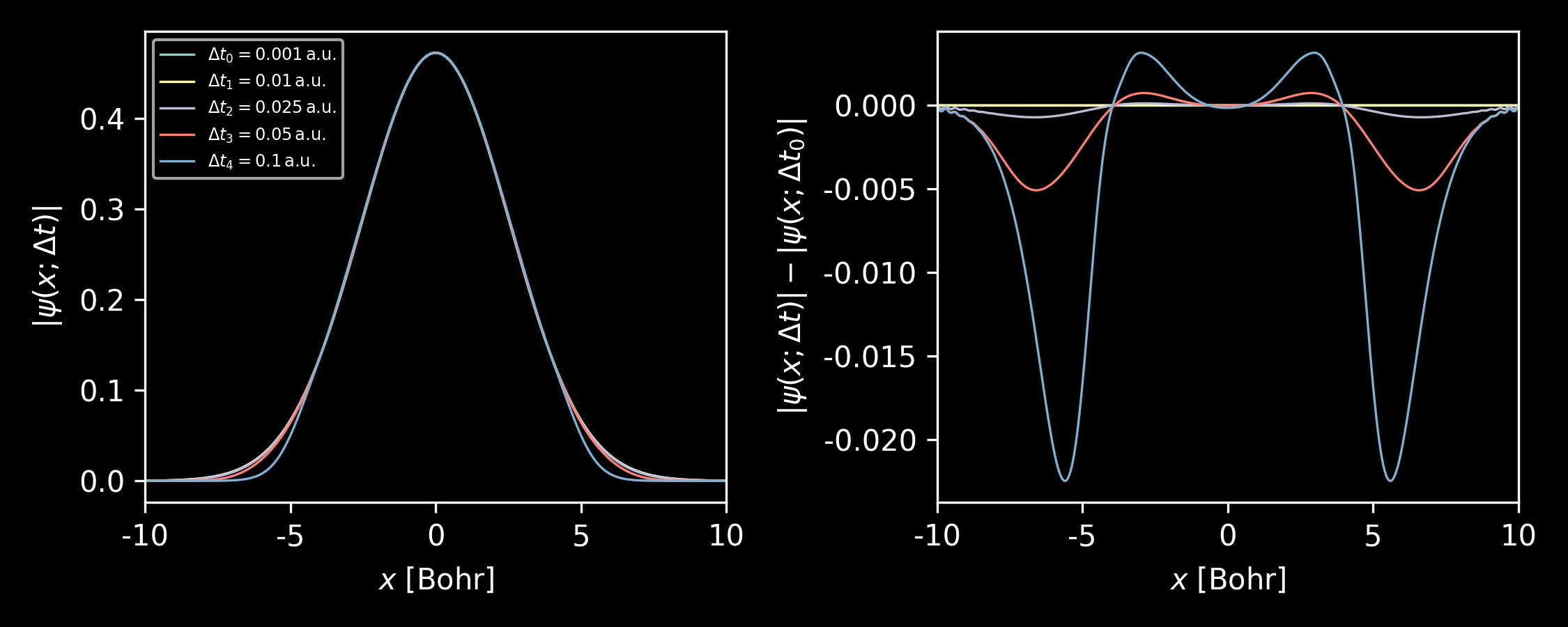
A rather important parameter for integrating the Schrödinger equation is the time step $\Delta t$. As can be seen below, with average wavepacket momentum $k_0 = 0$, the result from $\Delta t= 0.01$ already gives a reasonable result, as compared to that of $\Delta t = 0.001$.

Figure 1. Left: Wavefunctions at $t = 1.0\,$a.u. from Crank-Nicolson method with different time steps. Right: Differences of the wavefunctions. The average momentum of the Gaussian wavepacket $k_0 = 0$ and the width of the packet width $\sigma_x = 0.4$, both in atomic units. Figure generated by this script. As is well known that the Fourier transform of a Gaussian function is also a Gaussian, i.e.
\[\begin{equation} {\cal F}[\psi_0(x)](k) = c\cdot e^{-\frac{(k-k_0)^2}{2\sigma_k^2}}; \quad \sigma_k = 2\pi / \sigma_x \end{equation}\]where $c$ is a normalization factor. The above equation shows that the Gaussian wavepacket can be expanded by plane waves with amplitude also being a Gaussian. The spread of the plane wave momentum mainly locates within $k\in [k_0-\sigma_k, k_0 + \sigma_k]$. Therefore, by considering the plane waves with $k = k_0 + \sigma_k$, the time step can be approximated by
\[\begin{equation} \Delta t \approx 1 / E_k = \left[\frac{(k + \sigma_k)^2}{2}\right]^{-1} \end{equation}\]For $k_0 = 0$ and $\sigma_x = 0.4$, the equation gives $\Delta t = 0.008$, which is consistent with our test. Apparently, with larger wavepacket momentum $k_0$ and smaller packet width $\sigma_x$, the reasonable time step will become smaller.
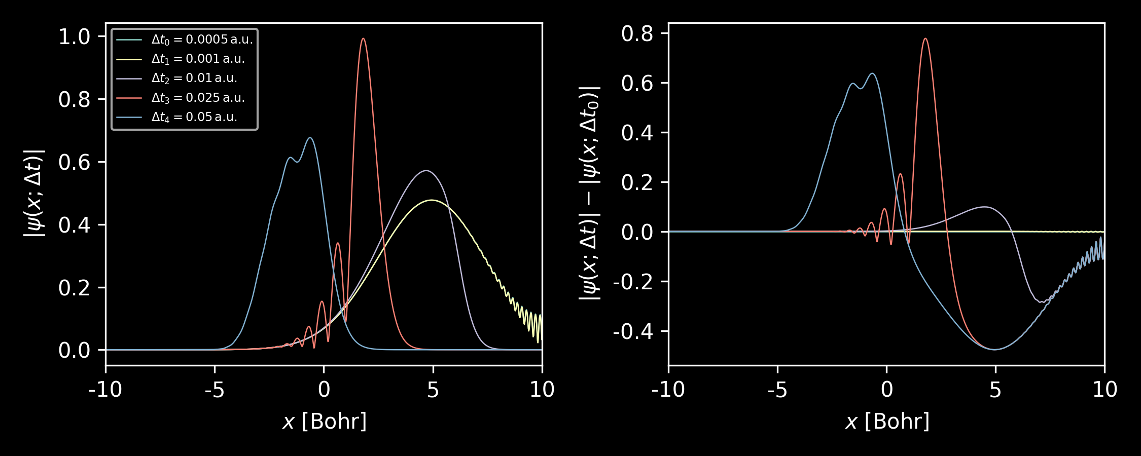
Figure 2. Left: Wavefunctions at $t = 1.0\,$a.u. from Crank-Nicolson method with different time steps. Right: Differences of the wavefunctions. The average momentum of the Gaussian wavepacket $k_0 = 10$, the width of the packet width $\sigma_x = 0.4$ and the converged time step is estimated to be $\Delta t = 0.003$, all in atomic units. -
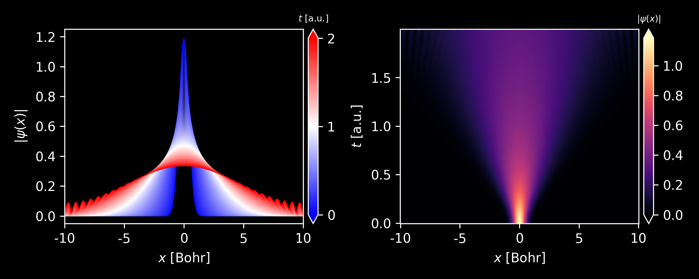
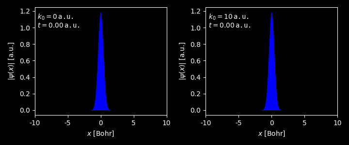
Evolution of the wavepacket with different average momentum $k_0$.
Figure 3. Evolution of the wavepacket with $k_0 = 0$. Generated by this script.
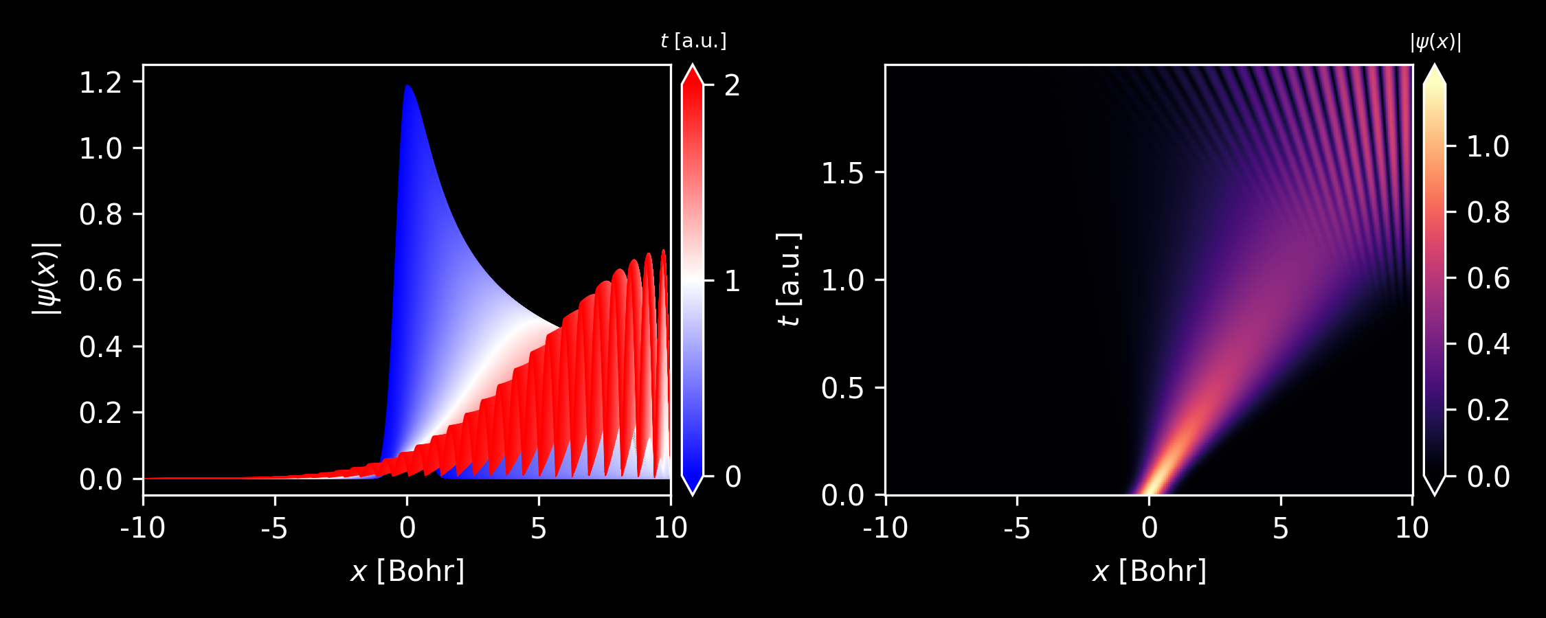
Figure 4. Evolution of the wavepacket with $k_0 = 1$. Generated by this script.
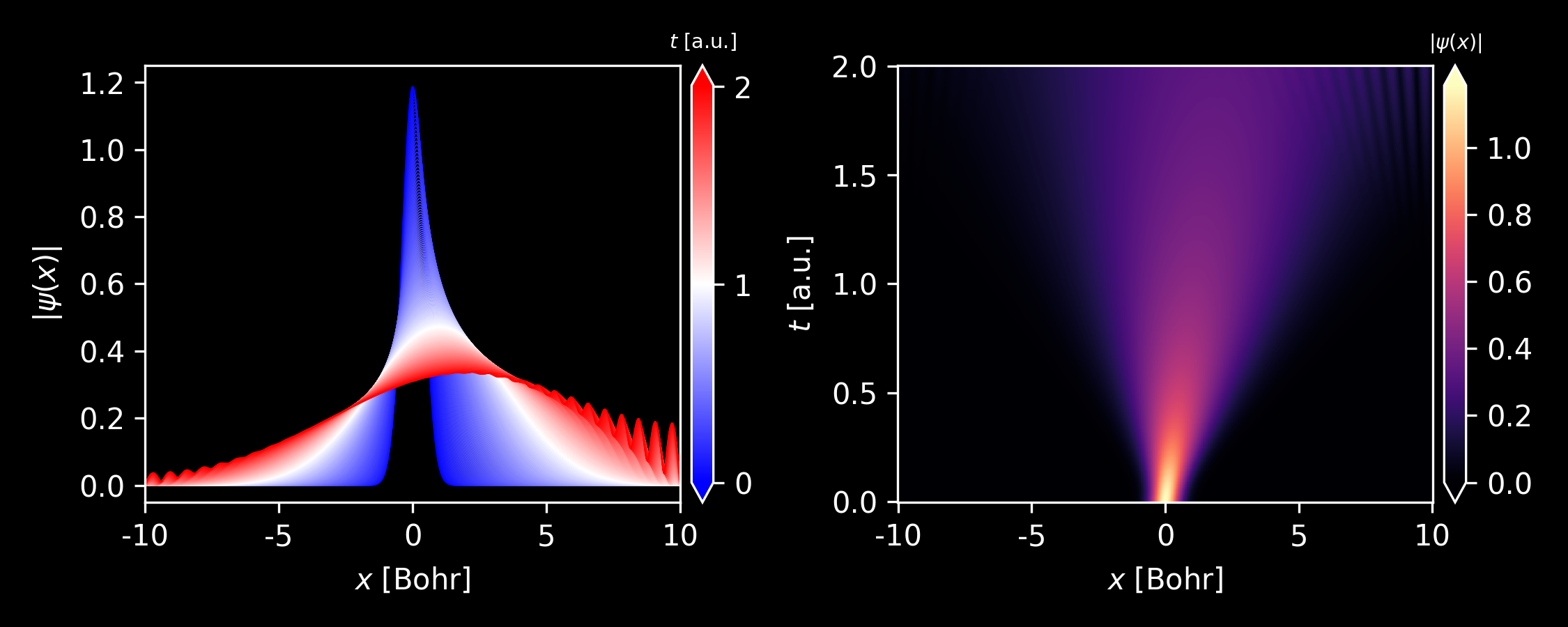
Figure 5. Evolution of the wavepacket with $k_0 = 5$. Generated by this script. -
Animation of time propagation of Gaussian wavepacket with different initial momenta $k_0 = 0$ and $k_0 = 10$ a.u.
Figure 6. Generated by matplotlib animation. -
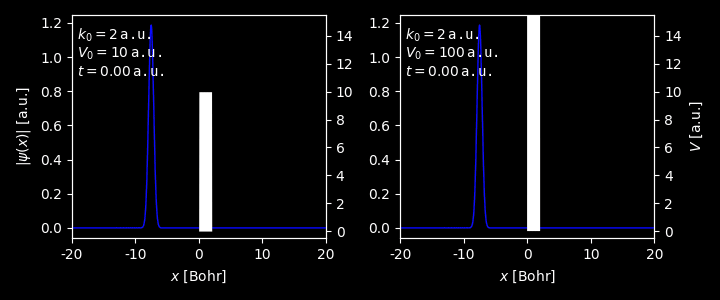
Animation of time propagation of Gaussian wavepacket in the existence of a finite barrier with different barrier height $V_0 = 10$ and $V_0 = 100$ a.u. The barrier width is set to 2 a.u.
Figure 7. Generated by matplotlib animation. As can be clearly seen, when the barrier height is modest (10 a.u.), quantum tunnelling can be observed. However, when the barrier is set to a rather high value (100 a.u.), tunneling can be hardly seen.
For solution to higher dimensional Schrödinger equation, one can referred to the QMsolve code. 5
Runge-Kutta Method
For an initial value equation,
\[\dfrac{\mathrm{d}y}{\mathrm{d}t} = f(t, y)\]The 4-th order Runge-Kutta (RK4) method6 gives
\[\begin{equation} y^{n+1} = y^n + \frac{1}{6}\cdot(k_1 + 2k_2 + 2k_3 + k_4) \end{equation}\]where
\[\begin{align} k_1 &= \Delta t \cdot f(t^n, y^n) \\ k_2 &= \Delta t \cdot f(t^n + \frac{\Delta t}{2}, y^n + \frac{k_1}{2}) \\ k_3 &= \Delta t \cdot f(t^n + \frac{\Delta t}{2}, y^n + \frac{k_2}{2}) \\ k_4 &= \Delta t \cdot f(t^n + \Delta t, y^n + k_3) \\ \end{align}\]The python code for the 1D Schrodinger equation using Runge-Kutta method can be written as follows.
1
2
3
4
5
6
7
8
9
10
11
12
13
14
15
16
17
18
19
20
21
22
23
24
25
26
27
28
29
30
31
def RungeKutta(psi0, V, x, dt, N=100, print_norm=False):
    '''
    4th-order Runge-Kutta method for the 1D Schrodinger equation.
    '''
    # No. of spatial grid points
    J  = x.size - 1
    dx = x[1] - x[0]

    # the external potential
    V = spa.diags(V)
    # the kinetic operator
    O = np.ones(J+1)
    T = (-1 / 2 / dx**2) * spa.spdiags([O, -2*O, O], [-1, 0, 1], J+1, J+1)
    U = -1j*(T + V)

    # Store all the wavefunctions
    PSI_t = np.zeros((J+1, N), dtype=complex)
    # the initial wavefunction
    PSI_t[:, 0] = psi0

    for n in range(N-1):
        k1 = dt * U.dot(PSI_t[:,n])
        k2 = dt * U.dot(PSI_t[:,n] + 0.5*k1)
        k3 = dt * U.dot(PSI_t[:,n] + 0.5*k2)
        k4 = dt * U.dot(PSI_t[:,n] + 1.0*k3)

        PSI_t[:,n+1] = PSI_t[:,n] + (k1 + 2*k2 + 2*k3 + k4) / 6.
        if print_norm:
            print(n, np.trapz(np.abs(PSI_t[:,n+1])**2, x))

    return PSI_t
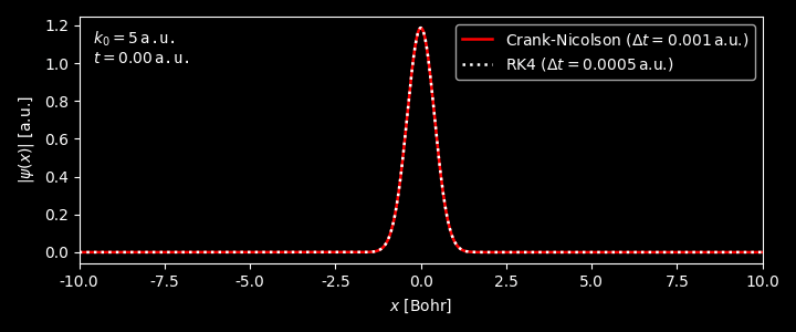
- As can be seen, although the results from RK4 and Crank-Nicolson method match fairly well, the time step for the RK4 method is much smaller than that used in the Crank-Nicolson method. For a larger time step, e.g. 0.0008, the norm of wavefunction from RK4 method will diverge.
Polynomial Methods
In the polynomial methods, the propagator ${\cal U}(\Delta t)$ is approximated by
\[\begin{equation} {\cal U}(\Delta t) = e^{-i{\cal H}\cdot\Delta t} \approx \sum_n a_n P_n({\cal H}) \end{equation}\]where $P_n(\cal H)$ is a polynomial of the Hamiltonian operator $\cal H$, whose operation on the wavefunction $\psi$ can be evaluated by interation of $\cal H$ on $\psi$. For example, if we know how to calculate ${\cal H}\cdot\psi$, then we can calculate ${\cal H}^2\cdot\psi = {\cal H}\cdot({\cal H}\cdot\psi)$ and finally ${\cal H}^n\cdot\psi$.
Chebyshev polynomials
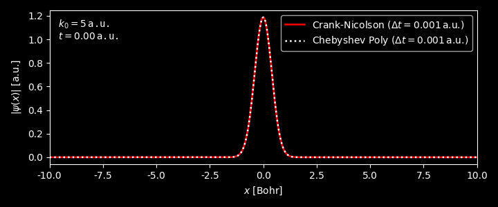
On can of course use Taylor expansion to expand ${\cal U}(\Delta t)$, however, a better choice is to use the Chebyshev polynomials. 7
\[\begin{equation} e^{-i{\cal H}\cdot \Delta t} = J_0(\tau) \cdot \mathbb{I} + \sum_{n=1}^\infty (-i)^n \, J_n(\tau) \, T_n(H) \end{equation}\]where $\mathbb{I}$ is the indentity operator, $J_n$ is the Bessel function of the first kind of order $n$,8 $T_n$ is the first-kind Chebyshev polynomial of degreen $n$. The dimensionless time $\tau$ and dimensionless Hamiltonian $H$ are defined as
\[\begin{equation} \tau = \|{\cal H}\| \cdot \Delta t, \qquad H = \dfrac{\cal H}{\|{\cal H}\|} \end{equation}\]The norm $\|\cdot\|$ is chosen such that $\|T_n(H)\|\le 1$ and $H \in [-1, 1]$ for all $n$. A reasonable choice is the maximum matrix element of $\|{\cal H}\| = {\cal H}_{max}$. As $J_n(\tau)| \le \tau^n / 2^n n!$, the series converges rapidly for any fixed $\tau$, therefore, we can truncate the expansion at some finite $n = N$.
Note how the dimensionless time $\tau$ depend on the time step $\Delta t$ and $\|{\cal H}\|$, which again depends on $\Delta x$ and $V$. As a result, for a chosen accuracy, the truncation $N$ also depends on the time and spatial step.
The numerical evaluation of the operators $T_n(H)$ is straightforward in view of the following recurrence relation:
\[\begin{align} T_0(H) &= \mathbb{I} \\ T_1(H) &= H \\ T_n(H) &= 2H\cdot T_{n-1}(H) - T_{n-2}(H) \end{align}\]As a result,
\[\begin{equation} \psi(t+\Delta t) \approx J_0(\tau)\cdot\psi_0(t) + 2\sum_{n=1}^N (-i)^n J_n(\tau) \psi_n(t) \end{equation}\]where
\[\begin{align} \psi_0(t) &= \psi(t) \\ \psi_1(t) &= H\cdot\psi_0(t) \\ \psi_n(t) &= 2H\cdot \psi_{n-1}(t) - \psi_{n-2}(t) \end{align}\]The python code implementation:
1
2
3
4
5
6
7
8
9
10
11
12
13
14
15
16
17
18
19
20
21
22
23
24
25
26
27
28
29
30
31
32
33
34
35
36
37
38
39
40
41
42
43
44
45
46
47
48
49
50
def ChebyshevPoly(psi0, V, x, dt, N=100, delta=1E-6, print_norm=False):
    '''
    Chebyshev polynomial expansion for the 1D Schrodinger equation.
    '''
    from scipy.special import j0, j1, jv

    # No. of spatial grid points
    J  = x.size - 1
    dx = x[1] - x[0]

    Hmax   = V.max() + (1 / dx**2)
    tau    = Hmax * dt

    # Jn_tau = np.r_[j0(tau), 2 * (-1j)**np.arange(1,Npoly) * jv(range(1,Npoly), tau)]
    Jn_tau = [j0(tau), -2j*j1(tau)]
    ii = 2
    while True:
        tmp = 2 * (-1j)**ii * jv(ii, tau)
        if np.abs(tmp) < delta:
            break
        Jn_tau += [tmp]
        ii += 1
    Npoly = len(Jn_tau)
    print("Chebyshev expansion truncated at N = {}.".format(Npoly))

    # the external potential
    V = spa.diags(V)
    # the kinetic operator
    O = np.ones(J+1)
    T = (-1 / 2 / dx**2) * spa.spdiags([O, -2*O, O], [-1, 0, 1], J+1, J+1)
    H = (T + V) / Hmax

    # Store all the wavefunctions
    PSI_t        = np.zeros((J+1, N), dtype=complex)
    PSI_ShebyExp = np.zeros((J+1, Npoly), dtype=complex)
    # the initial wavefunction
    PSI_t[:, 0] = psi0

    for n in range(N-1):
        PSI_ShebyExp[:,0] = PSI_t[:,n]
        PSI_ShebyExp[:,1] = H.dot(PSI_ShebyExp[:,0])
        for jj in range(2, Npoly):
            PSI_ShebyExp[:,jj] = 2*H.dot(PSI_ShebyExp[:,jj-1])
            PSI_ShebyExp[:,jj] -= PSI_ShebyExp[:,jj-2]

        PSI_t[:,n+1] = np.dot(PSI_ShebyExp, Jn_tau)
        if print_norm:
            print(n, np.trapz(np.abs(PSI_t[:,n+1])**2, x))

    return PSI_t
Lanczos Method
A different approach to approximately computing ${\cal U}(\Delta t)$ using only the action of ${\cal H}$ on the wavefunction $\psi$ is the Lanczos method, where a polynomial expansion is recursively created that builds an orthonormal basis in the Mth order Krylov subspace9 spanned by $\lbrace\psi, {\cal H}\psi, {\cal H}^2\psi,\ldots,{\cal H}^{M-1}\psi\rbrace$. The approximate solution is then given by projection of the exact solution to the Krylov subspace.10
-
Krylov Subspace and Lanczos Basis. The Mth order Krylov subspace with respect to $\cal H$ and $\psi$ is
\[{\cal K}_M({\cal H}, \psi) = \mathrm{span}\,\{\psi, {\cal H}\psi, {\cal H}^2\psi,\ldots,{\cal H}^{M-1}\psi\}\]that is, the space of all polynomials of $\cal H$ up to degree M-1 acting on $\psi$.
Gram-Schmidt orthogonalization is then used to build an orthonormal basis of this space (Lanczos basis): starting with $v_1 = \psi / \|\psi\|$ (or just $v_1 = \psi$ since $\psi$ is already normalized), it constructs $v_{k+1}$ recursively from $k=1,2,\ldots$ by orthogonzaling ${\cal H}\cdot v_k$ against the previous $v_j$ and normalizing:
\[\begin{align} V_{k+1} &= {\cal H}\cdot v_k - \sum_{j=1}^k H^L_{j,k}\,v_j \\[6pt] v_{k+1} &= V_{k+1} / \|V_{k+1}\| \\[9pt] H^L_{j,k} &= v_j^*\,{\cal H}\, v_k \end{align}\]By the Mth step, the method generates M orthonormal Lanzcos basis vectors $v_k$ and the M$\times$M matrix $H^L$.
-
Apparently, by multiplying $v_{k+1}^*$ and using the orthonormal conditions, one can get
\[\begin{equation} H^L_{k+1,k}\,v_{k+1} = V_{k+1} = {\cal H}\cdot v_k - \sum_{j=1}^k H^L_{j,k}\,v_j \end{equation}\] -
One can also readily see that $H^L_{l,k} = 0$ for $l - k > 1$, since
\[\begin{equation} H^L_{k+1,k}\,v^*_l\,v_{k+1} = H^L_{l,k} - \sum_{j=1}^k H^L_{j,k}\,v^*_l\,v_j = 0 \end{equation}\] -
For an Hermite Hamiltonian ${\cal H}$, the matrix $H^L$ is also an Hermite matrix, and since $H^L_{j,k} = 0$ for $j - k > 1$, one can readily see that $H^L$ is a tridiagonal Hermite matrix.
-
-
One then project the Hamiltonian $\cal H$ and the wavefunction $\psi$ on the Krylov subspace. The matrix representation of $\cal H$ is apparently $H^L$ and the representation of the wavefunction $\psi$ in the Kyrlov subspace is a column vector which can be expressed as
\[e_\ell = \begin{pmatrix}1, 0, 0, \ldots, 0 \end{pmatrix}^T\]The evolution of the wavefunction in the Krylov subspace can then be readily written as
\[\begin{align} e^\ell(\Delta t) &= e^{-iH^L\Delta t}\cdot e^\ell \\ &= U\, e^{-i E^L \Delta t} \, U^\dagger \cdot e^\ell \end{align}\]where $E^L$ is a diagonal matrix and $E^L = U^\dagger H^L U$.
-
One can then get the wavefunction in the original space by linear combination of the Lanczos basis. If we write the Lanczos basis as column vectors
\[V_M = \begin{pmatrix}v_1, v_2, v_3, \ldots, v_M\end{pmatrix}^T\]then
\[\psi(\Delta t) = e^\ell(\Delta t) \cdot V_m\] -
To summarize, the Lanzcos method can be written as
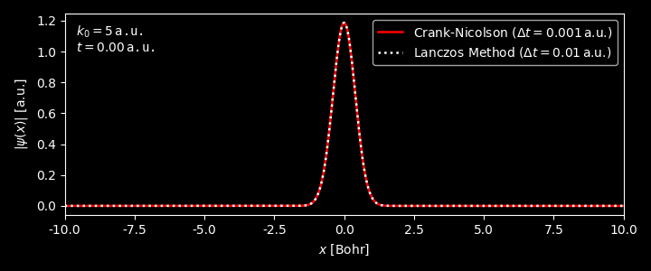
\[\psi(t+\Delta t) = e^{-i{\cal H}\Delta t}\cdot \psi(t) \approx V_M\cdot Ue^{-iE^L\Delta t}U^\dagger e_\ell\]Apparently, the time step $\Delta t$ depends on the dimension of the Krylov subspcae M, the larger the dimension M, the bigger the time step $\Delta t$.
The
pythoncode implementation of the Lanczos method follows.1 2 3 4 5 6 7 8 9 10 11 12 13 14 15 16 17 18 19 20 21 22 23 24 25 26 27 28 29 30 31 32 33 34 35 36 37 38 39 40 41 42 43 44 45 46 47 48 49 50 51 52 53 54 55 56 57 58 59 60 61 62 63 64 65
def Lanczos(psi0, V, x, dt, N=100, M=15, print_norm=False): ''' Lanczos method for the 1D Schrodinger equation. ''' from scipy.linalg import eigh # No. of spatial grid points J = x.size - 1 dx = x[1] - x[0] # the external potential V = spa.diags(V) # the kinetic operator O = np.ones(J+1) T = (-1 / 2 / dx**2) * spa.spdiags([O, -2*O, O], [-1, 0, 1], J+1, J+1) H = (T + V) # Store all the wavefunctions PSI_t = np.zeros((J+1, N), dtype=complex) # the initial wavefunction PSI_t[:, 0] = psi0 # orthonormal basis for the Krylov subspace Vlanc = np.zeros((J+1, M), dtype=complex) # Hamiltonian matrix in the Krylov subspace Hlanc = np.zeros((M, M), dtype=complex) # e1 e1 = np.r_[1, np.zeros(M-1)] for n in range(N-1): # Constructing: # 1. The Lanczos basis for the Krylov subspace: Vlanc # 2. The Hamiltonian matrix in the Lanczos basis: Hlanc Vlanc[:,0] = PSI_t[:,n] / np.sqrt(np.trapz(np.abs(PSI_t[:,n])**2, x)) Hlanc[0,0] = np.trapz(Vlanc[:,0].conj() * H.dot(Vlanc[:,0]), x) for k in range(M-1): Vlanc[:,k+1] = H.dot(Vlanc[:,k]) for j in range(k+1): if k - j <= 1: Vlanc[:,k+1] -= Hlanc[j,k] * Vlanc[:,j] Vlanc[:,k+1] /= np.sqrt(np.trapz(np.abs(Vlanc[:,k+1])**2, x)) Hlanc[k+1,k+1] = np.trapz(Vlanc[:,k+1].conj() * H.dot(Vlanc[:,k+1]), x) Hlanc[k+1,k] = np.trapz(Vlanc[:,k+1].conj() * H.dot(Vlanc[:,k]), x) Hlanc[k,k+1] = Hlanc[k+1,k].conj() # if n == 0: # np.savetxt('hlanc.dat', np.abs(Hlanc)) # Diagnolizing the matrix Hlanc and get the transformation matrix U, the # eigenvalues E E, U = eigh(Hlanc) # evolving the wavefunction in the Krylov subspace phi_lanc = np.matmul( np.matmul(U, np.matmul(np.diag(np.exp(-1j*dt*E)), U.conj().T)), e1 ) # PSI_t[:,n+1] = np.dot(Vlanc, phi_lanc) if print_norm: print(n, np.trapz(np.abs(PSI_t[:,n+1])**2, x)) return PSI_t
Split-operator Techniques
The split-operator technique approximates the unitary opertor by Suzuki-Trotter expansion, for example, in second-order
\[\begin{align} {\cal U}(\Delta t) &= e^{-i{\cal H} \Delta t} = e^{-i[\hat{T} + \hat{V}]\Delta t} \\[9pt] &\approx e^{-i\hat{T}\Delta t /2} e^{-i\hat{V}{\Delta t}} e^{-i\hat{T}\Delta t /2} + {\cal O}(\Delta t^3) \label{eq:so-potential-ref} \\[9pt] &\approx e^{-i\hat{V}\Delta t /2} e^{-i\hat{T}{\Delta t}} e^{-i\hat{V}\Delta t /2} + {\cal O}(\Delta t^3) \label{eq:so-kinetic-ref} \end{align}\]It takes advantage of the fact that the Hamiltonian is composed of two terms: the kinetic operator $\hat{T}$ being diagonal in Fourier space and the potential operator being diagonal in real space. Since the three exponentials can be computed exactly, it is always unitary and unconditionally stable, providing a very reliable second-order method. Note that Eq.\eqref{eq:so-potential-ref} and \eqref{eq:so-kinetic-ref} are equally legitimate, with the former also being referred to as “potential referenced” split-operator (potential operator sandwiched in the middle) and the latter “kinetic referenced” one.
Integrating the Schrödinger Equation
We will focus on the “kinetic referenced” split-operator in \eqref{eq:so-kinetic-ref}, since the wavefunctions are represented on grid points in real space and as a result we only have to perform TWO Fourier transforms (FT) at each time evolution step.
The wavefunction and the potential are represented on $D$-dimensional grid points with values on grid points being $\psi_j^n$ and $v_j$, where $j$ is the index for the grid point and should again be considered as a compound index, for example $(j, k, l)$ in 3D case. Let’s denote the wavefunction at time $t^n$ as $\Psi^n$ and the potential as $V$, which are D-dimensional arrays themself.
Every time integration step consists of three sub-steps of successive applicaton of the operator on the wavefunction:
-
Acting potential operator on the wavefunction by half time step.
\[\begin{equation} \Psi^{n, n+\frac{1}{2}} = \exp\left[ -i\frac{\Delta t}{2} V \right]\cdot\Psi^{n} \end{equation}\]As we have stated, $V$ is diagonal in real space (this does NOT mean that $V$ is a diagonal matrix), the $\cdot$ operation thus represents elementwise multiplicaton of the two arrays: $\exp[-i\frac{\Delta t}{2}\Psi^n]$ and $V$.
-
Acting the kinetic operator on the wavefunction by one full time step.
\[\begin{equation} \Psi^{n+1, n+\frac{1}{2}} = {\cal F}^{-1}\left[ \exp\bigl[ -i\Delta t T \bigr] \cdot {\cal F}\bigl[\Psi^{n, n+\frac{1}{2}}\bigr] \right] \end{equation}\]where ${\cal F}$ and ${\cal F}^{-1}$ means FT and inverse FT, repsectively. The kinetic operator is diagonal in Fourier space and is simply the kinetic energy of the plane waves $k^2 / 2$. The $\cdot$ operation is also an elementwise matrix multiplicaton.
-
Acting potential operator on the wavefunction by another half time step.
\[\begin{equation} \Psi^{n+1} = \exp\left[ -i\frac{\Delta t}{2} V \right] \cdot \Psi^{n+1, n+\frac{1}{2}} \end{equation}\]
The python code for split-opertor method is shown below.
1
2
3
4
5
6
7
8
9
10
11
12
13
14
15
16
17
18
19
20
21
22
23
24
25
26
27
28
29
30
31
32
33
34
35
36
37
38
39
40
41
42
43
44
45
46
47
48
def SplitOperatorKin(psi0, V, L, dt, N=100):
    '''
    Splitting technique for evolving the time-dependent Schrodinger equation.

    Kinetic referenced second-order Suzuki-Trotter expansion is used.
    '''

    from scipy.fft import fft, ifft, fftfreq

    psi0  = np.asarray(psi0)
    V     = np.asarray(V)
    ngrid = V.shape
    assert V.ndim == len(L)
    assert V.shape == psi0.shape

    # the kinetic operator
    ff = [fftfreq(n, 1/n) for n in V.shape]

    if V.ndim == 1:
        k2 = (2 * np.pi / L[0])**2 * ff[0]**2
    elif V.ndim == 2:
        kx, ky = np.meshgrid(ff[0], ff[1])
        k2 = (np.pi * 2 / L[0])**2 * kx**2 + \
             (np.pi * 2 / L[1])**2 * ky**2
    else:
        raise(NotImplementedError)

    # the kinetic operator by one time step
    # k**2 / 2 is the kinetic energy of the plane waves
    Ut_full = np.exp(-1j * dt * k2 / 2.)

    # the potential operator by half time step
    Uv_half = np.exp(-1j * dt * V / 2.)

    # Store all the wavefunctions
    PSI_t = np.zeros(psi0.shape + (N,), dtype=complex)
    # the initial wavefunction
    PSI_t[..., 0] = psi0

    for n in range(N-1):
        PSI_t[:,n+1] = Uv_half *\
            ifft(
                Ut_full * fft(
                    Uv_half * PSI_t[..., n]
                )
            )

    return PSI_t
In the figure below, we have applied both the Crank-Nicolson and Split-operator method on the propagation of 1D Gaussian wavepacket, with the external potential being $0$ for $x\in[0,L]$. The average momentum of the packet $k_0$ was set to be 5 a.u.
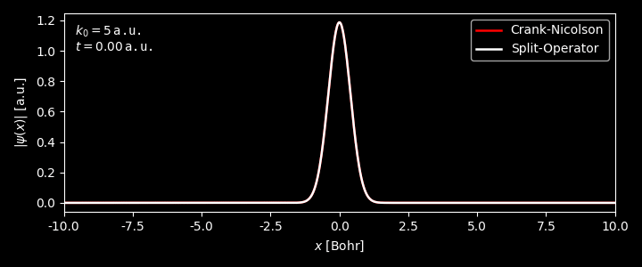
As can be clearly seen
-
For time $t \lesssim 0.8$ a.u., when the wavepacket is about to hit the boundary, the results from the two methods match reasonably well. Afterwards, the two methods start to differ significantly.
-
The reason lies in the fact that we are using zero-boundary condition in Crank-Nicolson method, as we have stated, while in the split-operator method we are implicitly adopting periodic-boundary condition when we performed Fourier transform. One can see that the wavefunction at both ends of the boundary from split-operator method are roughly the same. Before the wavefunction hits the boundary, the wavefucntion at both ends of the boundaries are zero, which does make a difference for the two boundary conditions.