
Numerov’s method
Numerov’s method1 (also called Cowell’s method) is a numerical method to solve ordinary differential equations of second order in which the first-order term does not appear. It is a fourth-order linear multistep method. The method is implicit, but can be made explicit if the differential equation is linear. Numerov’s method was developed by the Russian astronomer Boris Vasil’evich Numerov.
Given the differential equation of this form
\[\begin{equation} \frac{\mathrm{d}^2 y}{\mathrm{d} x^2} = -g(x)y(x) + s(x); \qquad x\in [a, b] \end{equation}\]where $g(x)$ and $s(x)$ are continuous function on the domain $[a, b]$. To derive the Numerov’s method, we first discretize the interval $[a, b]$ using equally spaced grid, where the grid space is $h = x_{n+1} - x_n$. We then proceed with the Taylor expansion of the function $y(x)$ around the point $x_n$:
\[\begin{align} y(x_{n+1}) &= y(x_n) + y{'}(x_n)h + \frac{y{''}(x_n)}{2!}h^2 + \frac{y{'''}(x_n)}{3!}h^3 \nonumber\\[6pt] &+ \frac{y{''''}(x_n)}{4!}h^4 + \frac{y{'''''}(x_n)}{5!}h^5 + \frac{y{''''''}(x_n)}{6!}h^6 + \ldots \end{align}\]Similarly, we have
\[\begin{align} y(x_{n-1}) &= y(x_n) - y{'}(x_n)h + \frac{y{''}(x_n)}{2!}h^2 - \frac{y{'''}(x_n)}{3!}h^3 \nonumber\\[6pt] &+ \frac{y{''''}(x_n)}{4!}h^4 - \frac{y{'''''}(x_n)}{5!}h^5 + \frac{y{''''''}(x_n)}{6!}h^6 + \ldots \end{align}\]By summing the two equations, we have
\[\begin{equation} y_{n+1} - 2y_n + y_{n-1} = h^2 y_n{''} + \frac{h^4}{12} y_n{''''} + {\cal{O}}(h^6) \end{equation}\]To get an expression for $y_n’’’’$, remember that $y_n’’ = -g_ny_n + s_n\equiv z_n $. By repeating the same procedure we did above
\[\begin{align} h^2 y_n'''' &= z_{n+1} - 2z_n + z_{n-1} + {\cal O}(h^4) \nonumber\\[6pt] &= -g_{n+1}y_{n+1} + s_{n+1} \nonumber\\[6pt] &\phantom{={}} +2g_{n}y_{n} - 2s_{n} \nonumber\\[6pt] &\phantom{={}} -g_{n-1}y_{n-1} + s_{n-1} + {\cal O}(h^4) \end{align}\]If we substitute this into the proceeding equation, we get
\[\begin{align} y_{n+1} - 2y_n + y_{n-1} &= h^2 (-g_ny_n + s_n) \nonumber \\[6pt] &\phantom{={}}+ \frac{h^2}{12} (-g_{n+1}y_{n+1} + s_{n+1} +2g_{n}y_{n} - 2s_{n} -g_{n-1}y_{n-1} + s_{n-1}) + {\cal{O}}(h^6) \end{align}\]or equivalently
\[\begin{equation} y_{n+1}(1 + {h^2\over12}g_{n+1}) - 2y_n(1 - {5h^2\over 12}g_n) + y_{n-1}(1 + {h^2\over12}g_{n-1}) = {h^2\over 12}(s_{n+1} + 10s_n + s_{n-1}) + {\cal O}(h^6) \end{equation}\]This yields the Numerov’s method if we ignore the term of order $h^6$.
\[\begin{align} y_{n+1} &= \frac{\displaystyle 2y_n(1 - {5h^2\over 12}g_n) - y_{n-1}(1 + {h^2\over12}g_{n-1}) + {h^2\over 12}(s_{n+1} + 10s_n + s_{n-1}) } {\displaystyle 1 + {h^2\over12}g_{n+1}} \nonumber\\[6pt] &= \frac{\displaystyle (12 - 10 f_n)y_n - y_{n-1}f_{n-1} + {h^2\over 12}(s_{n+1} + 10s_n + s_{n-1}) } {\displaystyle f_{n+1}} \end{align}\]where $f_n = 1 + {h^2\over 12} g_n$. It is easy to show that
\[\begin{equation} y_{n-1} = \frac{\displaystyle (12 - 10 f_n)y_n - y_{n+1}f_{n+1} + {h^2\over 12}(s_{n+1} + 10s_n + s_{n-1}) } {\displaystyle f_{n-1}} \end{equation}\]With this relation, we can now find the value of $y(x_{n+1})$ given two previous values $y(x_n)$ and $y(x_{n-1})$. All we have to do to find an approximate solution is to find the values $y(x_1)$ and $y(x_2)$ at the first two points $x_1$ and $x_2$, then we use the Numerov’s method to find the value of all following points in the interval $[a, b]$.
Case 1. Hydrogen-like atom
The Schrödinger equation for hydrogen-like atom is 2
\[\begin{equation} \left[ -{\hbar^2\over2m}\nabla^2 - {Ze^2\over4\pi\varepsilon_0 r} \right] \psi(\mathbf{r}) = E\psi(\mathbf{r}) \end{equation}\]Here, we assume that there is only one electron and thus neglecting the Coulomb interaction between the electrons. By variable separation, the wavefunction can be written as $\psi(\mathbf{r}) = {u(r)\over r} Y_{lm}({\hat r})$, where $Y_{lm}({\hat r})$ is the spherical harmonics and $u(r)$ follows the equation
\[\begin{equation} -{\hbar^2\over 2m} u'' + \left[ {\hbar^2\over 2m}{l(l+1)\over r^2}-{Ze^2\over4\pi\varepsilon_0 r} -E \right]u(r) = 0 \end{equation}\]Introducing the dimensionless variables
\[\newcommand{\AA}{\unicode{x212B}} \begin{align} x = {r \over a_0}; &\qquad a_0 = {4\pi\varepsilon_0\hbar^2\over me^2} \approx 0.529\,\AA \\[6pt] \epsilon = {E \over E_0}; &\qquad E_0 = {\hbar^2\over 2ma_0^2} = 1\,\text{Ry}\approx 13.60\,\text{eV} \end{align}\]where $a_0$ is the Bohr radius and $E_0$ is the Rydberg energy.
The equation for $u(r)$ then becomes
\[\begin{equation} u''(x) - \left[ {l(l+1)\over x^2} - {2Z\over x} - \epsilon \right]u(x) = 0 \end{equation}\]The boundary conditions are
\[\begin{equation} u(0) = 0; \qquad u(\infty) = 0 \end{equation}\]1. From known energy eigenvalue to the wavefunctions
As is well known that the energy levels of hydrogen-like atoms are
\[\begin{equation} E_n = - {Z^2 \over n^2}; \qquad n = 1, 2, 3, \ldots \end{equation}\]Let’s first show that given the correct energy levels, we can obtain the corresponding wavefunctions.
CLICK TO SHOW THE CODE!
1
2
3
4
5
6
7
8
9
10
11
12
13
14
15
16
17
18
19
20
21
22
23
24
25
26
27
28
29
30
31
32
33
34
35
36
37
38
39
40
41
42
43
44
45
46
47
48
49
50
51
52
53
54
55
56
57
58
59
60
61
62
63
64
65
66
67
68
69
70
71
72
73
74
75
76
77
78
79
80
81
82
83
84
85
86
87
88
89
90
91
92
93
94
#!/usr/bin/env python

import numpy as np
from scipy.integrate import odeint, simps

def radial_schrod_deriv(u, r, l, E, Z=1):
    '''
    The radial Schrödinger equation for hydrogen-like atom is

        u''(x) - [(l(l+1)/x^2) - (2Z/x) - E]u(x) = 0

    Since it is a second-order equation, i.e.

        y'' + g(x)y(x) = 0

    To use scipy.integrate.odeint, we can turn this equation into two
    first-order equation by defining a new dependent variables

        y'(x) = z(x)
        z'(x) = -g(x)y(x)

    Then we can solve this system of ODEs using "odeint" wit list.
    '''

    y, z = u

    return np.array([
        z,
        ((l*(l+1) / r**2) - (2*Z / r) - E) * y
    ])


def radial_wfc_scipy(r0, n=1, l=0, Z=1, direction='F', du=0.1):
    '''
    Get the radial wavefunction by integrating the equation with
    scipy.integrate.odeint.
    '''

    assert direction.upper() in ['F', 'B']

    E = -Z**2 / n**2

    # forward integration
    if direction.upper() == 'F':
        ur = odeint(radial_schrod_deriv, [0.0, du], r0, args=(l, E, Z))[:,0]

    # back integration
    else:
        ur = odeint(radial_schrod_deriv, [0.0, -du], r0[::-1], args=(l, E, Z))[:,0][::-1]

    # normalization
    ur /= np.sqrt(simps(ur**2, x=r0))

    return ur


def radial_wfc_numerov(r0, n=1, l=0, Z=1, du=0.001):
    '''
    Numerov algorithm

                  [12 - 10f(n)]*y(n) - y(n-1)*f(n-1)
        y(n+1) = ------------------------------------
                               f(n+1)

    where

        f(n) = 1 + (h**2 / 12)*g(n)

        g(n) = [E + (2*Z / x) - l*(l+1) / x**2]
    '''

    ur = np.zeros(r0.size)
    fn = np.zeros(r0.size)

    E      = -Z**2 / n**2
    ur[-1] = 0.0
    ur[-2] = du

    dr  = r0[1] - r0[0]
    h12 = dr**2 / 12.

    gn = (E + 2*Z / r0 - l*(l+1) / r0**2)
    fn = 1. + h12 * gn

    for ii in range(r0.size - 3, -1, -1):
        ur[ii] = (12 - 10*fn[ii+1]) * ur[ii+1] - \
                 ur[ii+2] * fn[ii+2]
        ur[ii] /= fn[ii]

    # normalization
    ur /= np.sqrt(simps(ur**2, x=r0))

    return ur
In the code above, we have defined two integration method to integrate the radial Schrödinger equation
-
radial_wfc_scipyusesodeintimplemented inscipy.3 -
radial_wfc_numerovuses the Numerov’s method. -
We implemented forward/backward integration scheme in
radial_wfc_scipyfunction, where forward integration means integrating from $u(0)$ and backward integraton starts from $u(\infty)$. -
Of course we can not integrate from $r=\infty$, we used a large enough cutoff $r_{c}$ and assumes $u(r_c) = 0$.
CLICK TO SHOW THE CODE!
1
2
3
4
5
6
7
8
9
10
11
12
13
14
15
16
17
18
19
20
21
22
23
24
25
26
27
28
29
30
31
32
33
34
35
36
37
38
39
40
41
42
43
44
45
46
47
48
49
50
51
52
53
54
55
56
57
58
59
60
61
62
63
64
65
66
67
68
69
70
71
72
73
74
75
76
77
78
################################################################################
# Define the radial grid
r0 = np.linspace(1E-10, 20, 500)

Z = 1
l = 0
n = 1

# forward integration from u(0)
ur1 = radial_wfc_scipy(r0, n, l, direction='F')
# backward integration from u(\infty)
ur2 = radial_wfc_scipy(r0, n, l, direction='B')
# backward integration from u(\infty) with Numerov method
ur3 = radial_wfc_numerov(r0, n, l)

################################################################################
import matplotlib as mpl
import matplotlib.pyplot as plt
plt.style.use('ggplot')

fig = plt.figure(
    figsize=(7.2, 3.0),
    dpi=300
)
axes = [plt.subplot(1,2,ii+1) for ii in range(2)]

################################################################################
ax = axes[0]

ax.plot(
    r0, ur1,
    ls='none',
    ms=4, marker='o', mfc='white', mew=1.0,
    zorder=1,
    label=r'Forward integration',
)

ax.plot(
    r0, ur2,
    ls='none',
    ms=4, marker='o', mfc='white', mew=1.0,
    zorder=1,
    label=r'Backward integration',
)
ax.plot(r0, 2*r0*np.exp(-r0), lw=1.0, color='cyan', zorder=2, label=r'Exact: $2r\cdot e^{-r}$')

ax.set_xlabel(r'$r$ [$a_0$]',   labelpad=5)
ax.set_ylabel(r'$u(r)$ [a.u.]', labelpad=5)

ylim = list(ax.get_ylim())
ylim[1] = 1.0
ax.set_ylim(ylim)
ax.legend(loc='best', fontsize='small')

#################################################################################
ax = axes[1]

ax.semilogy(
    r0, 2*r0*np.exp(-r0) - ur2,
    ls='-', alpha=0.8,
    zorder=1,
    label=r'scipy.integrate.odeint',
)

ax.semilogy(
    r0, 2*r0*np.exp(-r0) - ur3,
    ls=':', alpha=0.8,
    zorder=1,
    label=r'Numerov',
)
ax.legend(loc='lower right', fontsize='small')

ax.set_xlabel(r'$r$ [$a_0$]',   labelpad=5)
ax.set_ylabel(r'Error', labelpad=5)

plt.tight_layout()
plt.savefig('fig1.png')
plt.show()
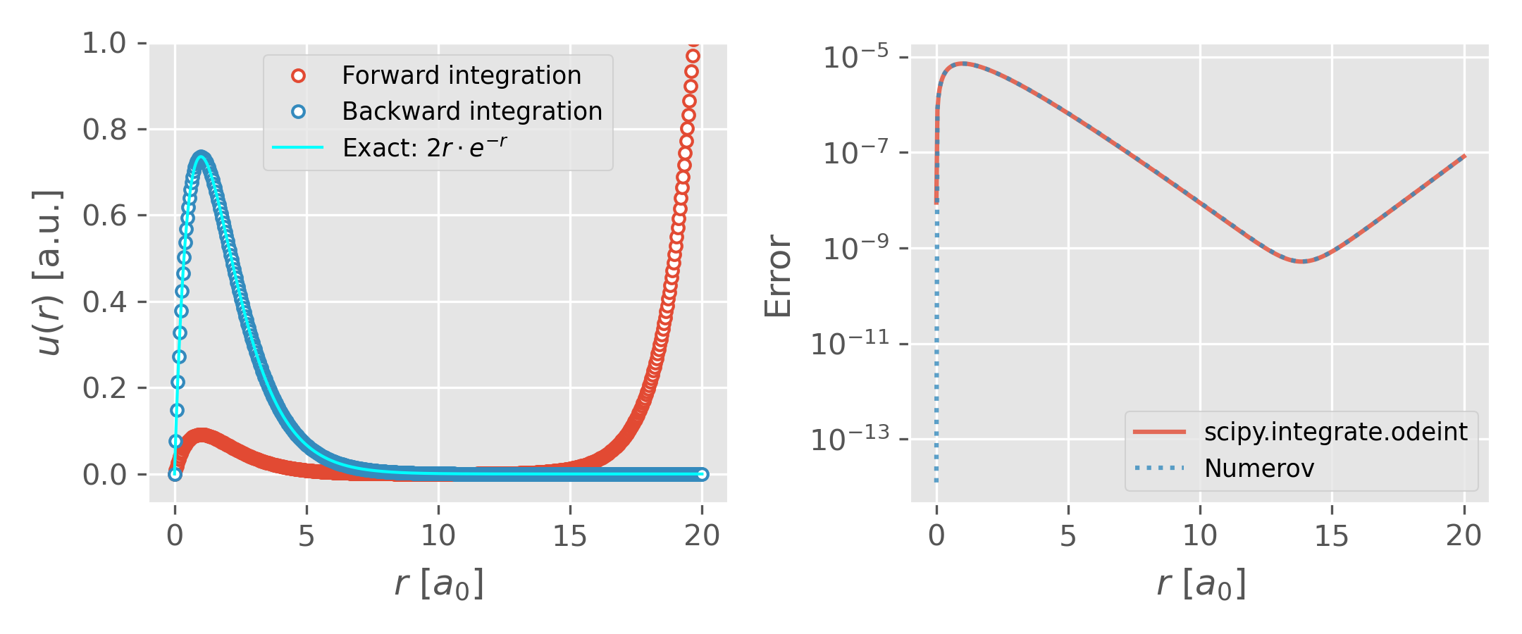
We then try to get the radial wavefunction of hydrogen ($Z=1$) with quantum number $n=1, l=0$. Some remarks here:
-
It turns out that the forward integration of the equation is not stable, as can be seen in the left panel of Figure 1.
-
It is better to use logarithmic mesh for radial variable rather than linear. Radial functions need smaller number of points in logarithmic mesh. For example, use
np.logspace(1E-6, 2, 500)to generate the radial grid and pass to theradial_wfc_scipyfunction. Note that Numerov’s method only support linear mesh, as can be seen in the method section.
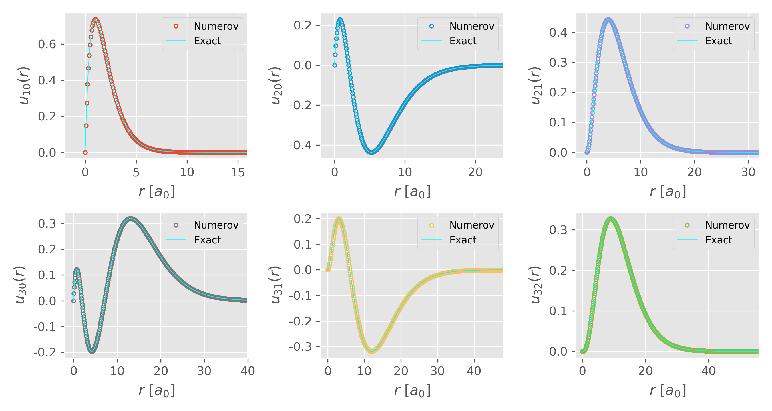
One can show that the Numerov’s method also works fine for higher excited states. For example, below we compare the radial wavefunction $u_{nl}(r)$ for $n=1,2,3$ obtained from Numerov method with the exact solutions. The script can be found here.
2. Unknown energy levels
If we don NOT know the correct energy levels, we can utilize the boundary condition to get the energy. Recall that the boundary condition is
\[\begin{equation} u(0) = 0; \qquad u(r_c) = 0 \end{equation}\]where $r_c$ is large enough so that $u(r_c) =0$. If $E_0$ corresponds to the correct energy level, when we integrate the radial wavefunction $u(r)$ from $r_c$ backward using Numerov’s method, we should get $u(0) = 0$. A deviation of the energy from $E_0$ will result in $u(0)\ne 0$. Therefore we can use the so called “shooting” method to get the correct energy. The basic procedure is
-
Start wite a guess energy, e.g. $E_1$. In practice, the guess energy should be smaller than the smallest potential energy. In our case, $E_1$ should be smaller than $-Z^2$. With the guess energy $E_1$, integrate the equation and get the value of the function at $r=0$, which we will denote as $u_1$. Meanwhile, Set another energy $E_2 = E_1$.
-
Increase $E_2$ by an amount $\delta E$ and get a new energy $E_2 = E_2 + \delta E$. Integrate the equation to get the value at $r=0$, which we will denote as $u_2$.
-
Go back to step 2 if $u_1 * u_2 > 0$.
-
At this step, we should have the correct energy enclosed in $[E_1, E_2]$. Use root finding method, e.g.
scipy.optimize.brentqto get the correct energy.
CLICK TO SHOW THE CODE!
1
2
3
4
5
6
7
8
9
10
11
12
13
14
15
16
17
18
19
20
21
22
23
24
25
26
27
28
29
30
31
32
33
34
35
36
37
38
39
40
41
42
43
44
45
46
47
48
49
50
51
52
53
54
55
56
57
58
59
60
61
62
63
#!/usr/bin/env python

import numpy as np
from scipy.integrate import odeint, simps
from scipy.optimize import brentq


def radial_wfc_at0(E, r0, n=1, l=0, Z=1, du=0.01):
    '''
    Numerov algorithm

                  [12 - 10f(n)]*y(n) - y(n-1)*f(n-1)
        y(n+1) = ------------------------------------
                               f(n+1)

    where

        f(n) = 1 + (h**2 / 12)*g(n)

        g(n) = [E + (2*Z / x) - l*(l+1) / x**2]

    here, we use reverse integration from the other end.
    '''
    ur = np.zeros_like(r0)
    ur[-1] = 0.0
    ur[-2] = du

    dr  = r0[1] - r0[0]
    h12 = dr**2 / 12.
    gn  = E + 2*Z / r0 - l*(l+1) / r0**2
    fn  = 1. + h12 * gn

    for ii in range(gn.size - 3, -1, -1):
        ur[ii] = (12 - 10*fn[ii+1]) * ur[ii+1] - \
                 ur[ii+2] * fn[ii+2]
        ur[ii] /= fn[ii]

    # normalization
    ur /= np.sqrt(simps(ur**2, x=r0))

    # now extrapolate the wavefunction to u(0)
    # the first derivative equals at ur[0]
    # (u0 - ur[0]) / (0 - r0[0]) = (ur[1] - ur[0]) / (r0[1] - r0[0])
    u0 = ur[0] + (ur[1] - ur[0]) * (0 - r0[0]) / dr

    return u0


if __name__ == "__main__":
    r0 = np.linspace(1E-6, 30, 3000)

    E_lower = E_upper = -1.1
    dE      = 0.10
    u1      = radial_wfc_at0(E_lower, r0, n=1)

    while True:
        E_upper += dE
        u2 = radial_wfc_at0(E_upper, r0, n=1)
        if u1 * u2 < 0:
            break

    E = brentq(radial_wfc_at0, E_lower, E_upper, args=(r0, 1, 0, 1, 0.001))
    print(E)