Molecular Dynamics at Constant Temperature

Canonical Ensemble

In a canonical ensemble, the particle number $N$, the volume $V$ and the temperature $T$ are fixed. The temperature of the system is connected to the averaged kinetic energy via

\[\begin{equation} \frac{3}{2} N k_B T = \langle E_{\mathrm{kin}} \rangle \end{equation}\]

Although the temperature and the average kinetic energy are fixed, the instantaneous kinetic energy fluctuates and with it the velocities of the particles. The instantaneous kinetic energy is often used to define the instantaneous temperature $T_\mathrm{in}$ by

\[\begin{equation} k_B T_{\mathrm{in}} = {2\over 3N} E_{\mathrm{kin}} \end{equation}\]

Note that in the microcanonical ensemble ($NVE$), the termperature is defined as $1 / T = \partial S /\partial E$. There is NO connection between the average kinetic energy and temperature.

In equilibrium, the relative variance of the instantaneous termperature fluctuation in a canonical ensemble is¹

\[\begin{equation} \label{eq:temperature_var} \frac{ \langle \Delta T^2 \rangle }{T^2} = \frac{ \langle (T_k - T)^2 \rangle }{ T^2 } = {2 \over 3N} \end{equation}\]

where $T = \langle T_k \rangle$ and $N$ is the number of atoms. In the thermodynamic limit ($N \to \infty$ and $V \to \infty$ while $N/V = \mathtt{const}$), the fluctuation is negligible. The fluctuation to become negligible in the thermodynamic limit is a general result, thus we are always at liberty to choose the ensemble that is most convenient for a particular problem and still obtain the same macroscopic observables. It must be stressed, however, this freedom only exists in thermodynamic limit. Note, Eq. \eqref{eq:temperature_var} can be used to check whether the simulation has reached equilibrium.

There are essentially three classes of method to control temperature in an MD simulation:²

Velocity scaling method (e.g. velocity rescaling and Berendsen thermostat)
Stochastic thermostat (e.g., Andersen thermostat, Langevin thermostat)
“Extended Lagrangian” formalisms (e.g., Nosé-Hoover thermostat, Nosé-Hoover Chain)

Velocity Rescaling

Stochastic Thermostat

Andersen Thermostat

A few remarks on the collision frequency:

An arbitrarily non-zero collision frequency are sufficient to guarantee in principle the generation of a canonical ensemble.
Too small values (loose coupling) may cause a poor temperature control. The canonical distribution will only be obtained after very long simulation times. In this case, systematic energy drifts due to accumulation of numerical errors may interfere with the thermostatization.
Too large values for the collision frequency (tight coupling) may cause the velocity reassignments to perturb heavily the dynamics of the system.

Pros and Cons

Langevin Thermostat

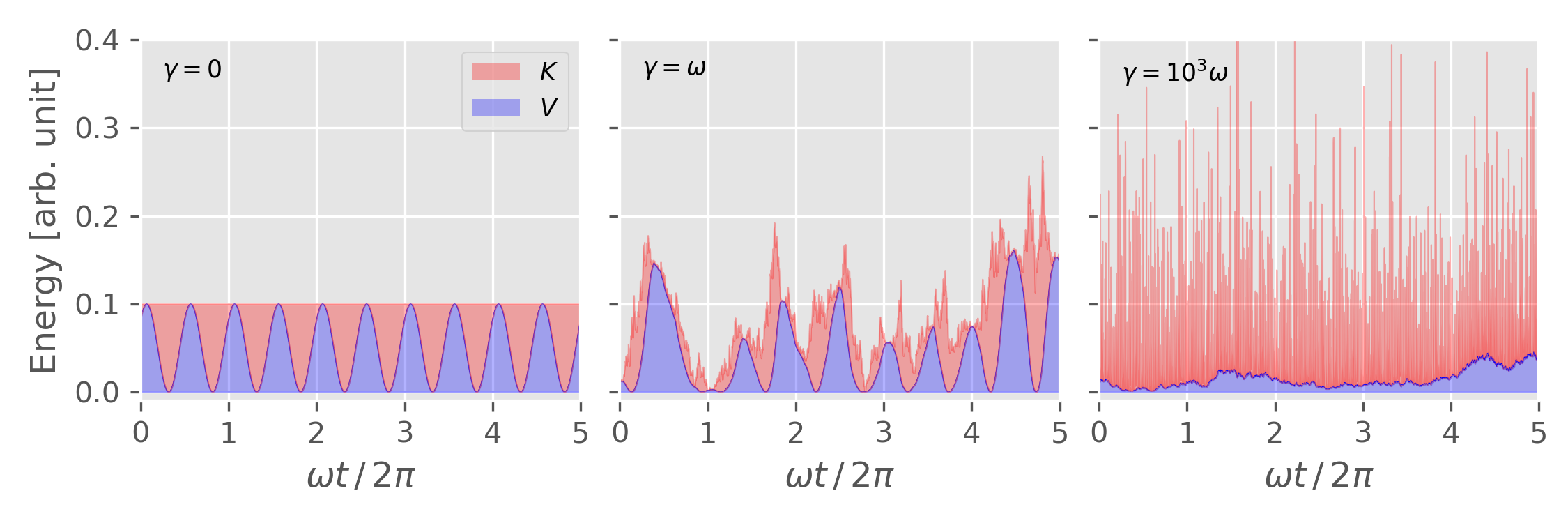
The equation of motion for Langevin dynamics is

\[\begin{equation} \label{eq:langevin_eom} m\frac{\mathrm{d}^2 \mathbf{r}_i}{\mathrm{d} t^2} = -\nabla V(\mathbf{r}_1,\ldots,\mathbf{r}_N) - \gamma m \mathbf{v}_i + \mathbf{R}_i \end{equation}\]

Velocity-Verlet algorithm for Langevin thermostats

\[\begin{align} \mathbf{v}_i(t + {\delta t\over 2}) &= \mathbf{v}_i(t) + {\delta t \over 2m} \left[ \mathbf{F}_i - \gamma m \mathbf{v}_i \right] + \mathbf{R}_i \end{align}\]

CLICK TO SHOW THE CODE!

#!/usr/bin/env python
# -*- coding: utf-8 -*-

import numpy as np


def harmonic_pot(x, m=1, omega=1):
    '''
    The harmonic potential
    '''

    return 0.5 * m * omega**2 * x**2

def harmonic_for(x, m=1, omega=1):
    '''
    The force of harmonic potential
    '''

    return - m * omega**2 * x

def Ekin(v, m=1):
    '''
    The force of harmonic potential
    '''

    return 0.5 * m * v**2

def log(x, v, m=1, omega=1):
    '''
    '''

    print("{:20.8E} {:20.8E} {:20.8E} {:20.8E} {:20.8E}".format(
        x, v,
        Ekin(v, m), 
        harmonic_pot(x, m, omega),
        harmonic_pot(x, m, omega) + Ekin(v, m)
    ))


def vv(x0, v0, f0=None, m=1, omega=1, dt=0.01, nsteps=1000):
    '''
    Velocity Verlet integration
    '''

    if f0 is None:
        f0 = harmonic_for(x0, m, omega)

    log(x0, v0, m, omega)

    for ii in range(nsteps):
        # x(t+dt) = x(t) + v(t) * dt + f(t) * dt**2 / (2*m)
        x1 = x0 + v0 * dt + f0 * dt**2 / (2*m)
        # f(t+dt)
        f1 = harmonic_for(x1, m, omega)
        # v(t+dt) = v(t) + dt * (f(t) + f(t+dt)) / (2*m)
        v1 = v0 + dt * (f1 + f0) / (2*m)

        log(x1, v1, m, omega)
        x0, v0, f0 = x1, v1, f1

def langevin(x0, v0, T, gamma, dt=0.01, f0=None, m=1, omega=1, nsteps=1000):
    '''
    Velocity Verlet integration for Nose-Hoover thermostat
    '''

    if f0 is None:
        f0 = harmonic_for(x0, m, omega)

    log(x0, v0, m, omega)

    # the random force is sampled from Gaussian distribution with variance
    # sigma**2
    sigma = np.sqrt(2 * m * gamma * T / dt)
    R0    = np.random.standard_normal() * sigma

    # 0, 1, 2 represents t, t + 0.5*dt, and t + dt, respectively
    for ii in range(nsteps):
        v1 = v0 + 0.5 * dt * (f0 - gamma * m * v0 + R0) / m
        x2 = x0 + v1 * dt
        f2 = harmonic_for(x2, m, omega)
        R2 = np.random.standard_normal() * sigma
        v2 = v1 + 0.5 * dt * (f2 - gamma * m * v1 + R2) / m

        log(x2, v2, m, omega)
        x0, v0, f0, R0 = x2, v2, f2, R2

if __name__ == "__main__":
    T0 = 0.1
    v0 = np.sqrt(2*T0)
    x0 = 0.0
    dt = 0.01
    N  = 10000

    np.random.seed(20210605)

    langevin(x0, v0, T=T0, gamma=0 / (np.pi * 2), dt=dt, nsteps=N)
    langevin(x0, v0, T=T0, gamma=1 / (np.pi * 2), dt=dt, nsteps=N)
    langevin(x0, v0, T=T0, gamma=1000 / (np.pi * 2), dt=dt, nsteps=N)

T0 = 0.1
dt = 0.1
x0 = 0.0
v0 = np.sqrt(2 * T0)
N  = 10000

np.random.seed(20210605)
langevin(x0, v0, T=T0, gamma=1 / (np.pi * 2), dt=dt, nsteps=N)

**Figure 1.** Phase space distribution of 1D harmonic oscillator obtained from MD simulation with the Langevin thermostat. The friction term was chosen to match the frequency of the harmonic oscillator. The parameters for the simulation are $T = 0.1; dt = 0.1, N = 10000; x_0 = 0; v_0 = \sqrt{2T}; \gamma = {1\over 2\pi}$. Figure plotted using this script with this input data.

**Figure 2.** Potential energy and kinetic energy from Langevin dynamics with different friction coefficients. Figure plotted using this script with this input data.

Extended Lagrangian Method

Nosé-Hoover Thermostat

In Nosé-Hoover’s approach³⁴, an additional “agent” is introduced into the system to “check” whether the instantaneous kinetic energy is higher or lower than the desired temperature and then scales the velocities accordingly, effectively acting as a heat reservoir. Denoting this extra variable as $s$ and its conjugate momentum as $p_s$, the Nosé Hamiltonian for the extended system takes the form⁵

\[\begin{equation} \label{eq:nose_hamil} {\cal H}_N = \sum_{i=1}^{N} \frac{\mathbf{p}_i^2}{2m_i s^2} + V(\mathbf{r}_1,\ldots,\mathbf{r}_N) + \frac{p_s^2}{2Q} + gk_BT\ln{s} \end{equation}\]

where $Q$ is “thermal inertia”, which determines the time scale on which the extended variable acts. Note that $Q$ is NOT a mass! Rather, it has unit of $[\mathtt{Energy} \times \mathtt{Time}^2]$, or equivalently $[\mathtt{Mass} \times \mathtt{Length}^2]$. The logarithmic term is the potential for the extra variable $s$.

On the other hand, the Hamiltonian of the real system is defined as

\[\begin{equation} \label{eq:real_hamil} {\cal H}(\mathbf{p}', \mathbf{r}') = \sum_{i=1}^N \frac{\mathbf{p'}^2}{2m_i} + V(\mathbf{r}'_1,\ldots,\mathbf{r}'_N) \end{equation}\]

where the prime is used to indicate the real variables. Frow now on, we shall refer to the primed variables as real variables and those in the Nosé system as virtual variables. The real and virtual variables are related through¹³

\[\begin{align} \mathbf{r}' &= \mathbf{r} \\[6pt] \mathbf{p}' &= \mathbf{p} / s \\[6pt] s' &= s \\[6pt] p_s' &= p_s / s \\[6pt] \mathrm{d}t' &= \mathrm{d}t / s \label{eq:r2v_dt} \\[6pt] \end{align}\]

From Eq.\eqref{eq:r2v_dt}, it follows that $s$ can be interpreted as a scaling factor of the time step. In addition, the real and virtual times $\tau’$ and $\tau$ are related by

\[\begin{equation} \label{eq:r2v_time_int} \tau' = \int_0^{\tau} {1 \over s(t)}\, \mathrm{d}t \end{equation}\]

The partition function of the extended system¹³

\[\begin{align} Z_N &= {1 \over N!} \int \mathrm{d} p_s \, \mathrm{d} s \, \mathrm{d} \mathbf{p}^N \, \mathrm{d} \mathbf{r}^N \, \,\delta ({\cal H}_N - E) \nonumber \\[6pt] &= {1 \over N!} \int \mathrm{d} p_s \, \mathrm{d} s \, \mathrm{d} \mathbf{p'}^N \, \mathrm{d} \mathbf{r}^N \nonumber \\[6pt] &\phantom{={}} s^{3N} \times \delta \left[ \sum_{i=1}^{N} \frac{\mathbf{p'}_i^2}{2m_i} + V(\mathbf{r}_1,\ldots,\mathbf{r}_N) + \frac{p_s^2}{2Q} + gk_BT\ln{s} - E \right] \label{eq:nose_part_func} \end{align}\]

For a $\delta$-function of a function $h(s)$, we have this relation

\[\begin{equation} \label{eq:delta_function_relation} \delta[h(s)] = \frac{\delta(s - s_0)}{|h'(s_0)|} \end{equation}\]

where $h(s)$ is a function that has single root at $s_0$. Substitute Eq. \eqref{eq:delta_function_relation} into Eq. \eqref{eq:nose_part_func}, we get the following equation

\[\begin{align} Z_N &= {1 \over N!} \int \mathrm{d} p_s \, \mathrm{d} s \, \mathrm{d} \mathbf{p'}^N \, \mathrm{d} \mathbf{r}^N \nonumber \\[6pt] &\phantom{={}} {\beta s^{3N+1} \over g} \times \delta \left\{ s - \exp\left[ -\beta { {\cal H}(\mathbf{p}', \mathbf{r}) + p_s^2 / (2Q) - E \over g} \right] \right\} \nonumber \\[6pt] &= {1 \over N!} {\beta \exp[(3N+1)E/g] \over g} \int \mathrm{d} p_s \exp \left[ -\beta{3N+1 \over g} {p_s^2 \over 2Q} \right] \nonumber \\[6pt] &\phantom{={}} \times \int \mathrm{d} \mathbf{p'}^N \, \mathrm{d} \mathbf{r}^N \exp \left[ -\beta {3N+1 \over g} {\cal H}(\mathbf{p}', \mathbf{r}) \right] \nonumber \\[6pt] &= C {1 \over N!} \int \mathrm{d} \mathbf{p'}^N \, \mathrm{d} \mathbf{r}^N \exp \left[ -\beta {3N+1 \over g} {\cal H}(\mathbf{p}', \mathbf{r}) \right] \label{eq:nose_part_func_final} \end{align}\]

For a physical quantity $\cal A$ that depends on $\mathbf{p}’$ and $\mathbf{r}$, the microcanonical ensemble average of ${\cal A}$ in the extended system is given by

\[\begin{align} \langle {\cal A}(\mathbf{p}/s, \mathbf{r}) \rangle_{\mathrm{Nosé}} &= \frac{ \displaystyle \int \mathrm{d} \mathbf{p'}^N \, \mathrm{d} \mathbf{r}^N \, {\cal A}(\mathbf{p}', \mathbf{r}) \exp \left[ -\beta {3N+1 \over g} {\cal H}(\mathbf{p}', \mathbf{r}) \right] }{ \displaystyle \int \mathrm{d} \mathbf{p'}^N \, \mathrm{d} \mathbf{r}^N \, \exp \left[ -\beta {3N+1 \over g} {\cal H}(\mathbf{p}', \mathbf{r}) \right] } \nonumber \\[6pt] &= \frac{ \displaystyle {1 \over N!} \int \mathrm{d} \mathbf{p'}^N \, \mathrm{d} \mathbf{r}^N \, {\cal A}(\mathbf{p}', \mathbf{r}) \exp \left[ -\beta {\cal H}(\mathbf{p}', \mathbf{r}) \right] }{ \displaystyle {1 \over N!} \int \mathrm{d} \mathbf{p'}^N \, \mathrm{d} \mathbf{r}^N \, \exp \left[ -\beta {\cal H}(\mathbf{p}', \mathbf{r}) \right] } \nonumber \\[6pt] & = \langle {\cal A}(\mathbf{p}', \mathbf{r}) \rangle_{\mathrm{NVT}} \label{eq:nose_ensemble_average} \end{align}\]

where in the second line, we have chosen $g = 3N + 1$.

Eq. \eqref{eq:nose_ensemble_average} indicates that the canonical ensemble average of a centain physical quantity ${\cal A}(\mathbf{p}’, \mathbf{r})$ in a real system with Hamiltonian ${\cal H}(\mathbf{p}’, \mathbf{r})$, which we denote as $\langle {\cal A}(\mathbf{p}’, \mathbf{r}) \rangle_{\mathrm{NVT}}$, is equivalent to the microcanonical ensemble average of ${\cal A}(\mathbf{p}/s, \mathbf{r})$ in the extended Nosé system.

At this point, one can clearly see that the logarithmic form of the potential ($gk_BT \ln s$) is essential in the derivation of Eq. \eqref{eq:nose_part_func_final} and \eqref{eq:nose_ensemble_average}.

EOM in virtual variables

With the quasi-ergodic hypothesis, i.e. time average equals ensemble average, we have

\[\begin{equation} \label{eq:ergodic_hypo} \langle {\cal A}(\mathbf{p}', \mathbf{r}) \rangle_{\mathrm{NVT}} = \langle {\cal A}(\mathbf{p}/s, \mathbf{r}) \rangle_{\mathrm{Nosé}} = \lim_{\tau \to \infty} {1\over\tau} \int_0^\tau {\cal A}\left(\mathbf{p}(t)/s(t), \mathbf{r}(t)\right)\, \mathrm{d}t \end{equation}\]

We can thus proceed by generating a trajectory following the equations of motion (EOM) of the extended system, and get the canonical ensemble average of $\cal A$ in the real system by averaging over the trajectory according to Eq.\eqref{eq:ergodic_hypo}. From the Nosé Hamiltonian (Eq.\eqref{eq:nose_hamil}), the EOM in virtual variables are given by

\[\begin{align} \frac{\mathrm{d} \mathbf{r}_i}{\mathrm{d} t} &= {\partial\, {\cal H}_N \over \partial\, \mathbf{p}_i} = \frac{\mathbf{p}_i}{m_i s^2} \label{eq:virtual_eom_1}\\[6pt] \frac{\mathrm{d} \mathbf{p}_i}{\mathrm{d} t} &= -{\partial\, {\cal H}_N \over \partial\, \mathbf{r}_i} = -\frac{\partial\, V(\mathbf{r}_1,\ldots,\mathbf{r}_N)}{\partial\,\mathbf{r}_i} \label{eq:virtual_eom_2}\\[6pt] \frac{\mathrm{d} s}{\mathrm{d} t} &= {\partial\, {\cal H}_N \over \partial\, p_s} = {p_s \over Q} \label{eq:virtual_eom_3}\\[6pt] \frac{\mathrm{d} p_s}{\mathrm{d} t} &= -{\partial\, {\cal H}_N \over \partial\, s} = {1\over s}\left[\sum_i {\mathbf{p}_i^2\over m_i s^2} - gk_B T\right]\label{eq:virtual_eom_4} \end{align}\]

Note that $g = 3N + 1$ in Eq.\eqref{eq:virtual_eom_4}.

EOM in real variables

The last equivalence of Eq.\eqref{eq:ergodic_hypo} is done by sampling data points at integer multiples of virtual time step $\mathrm{d}t$. According to Eq.\eqref{eq:r2v_dt}, this means that the real time step $\mathrm{d}t’$ is fluctuating. Using Eq.\eqref{eq:r2v_time_int}, the time average of $\cal A$ in the real time $t’$ can be written

\[\begin{align} &\lim_{\tau' \to \infty} {1\over\tau'} \int_0^{\tau'} {\cal A}\left(\mathbf{p}(t')/s(t'), \mathbf{r}(t')\right)\, \mathrm{d}t' \nonumber\\[6pt] &= \lim_{\tau' \to \infty} {\tau \over \tau'} {1\over\tau} \int_0^\tau { {\cal A}\left(\mathbf{p}(t)/s(t), \mathbf{r}(t)\right) / s(t)}\, \mathrm{d}t \nonumber \\[6pt] &= \frac{ \displaystyle \lim_{\tau \to \infty} {1\over\tau} \int_0^\tau { {\cal A}\left(\mathbf{p}(t)/s(t), \mathbf{r}(t)\right) / s(t)}\, \mathrm{d}t \nonumber }{ \displaystyle \lim_{\tau \to \infty} {1\over\tau} \int_0^\tau {1\over s(t)}\, \mathrm{d}t \nonumber } \\[6pt] &= \frac{ \displaystyle \langle { {\cal A}(\mathbf{p}/s, \mathbf{r}) / s } \rangle_{\mathrm{Nosé}} }{ \langle { 1 / s } \rangle_{\mathrm{Nosé}} } \label{eq:real_time_aver} \end{align}\]

Consider again the Nosé partition function Eq.\eqref{eq:nose_part_func}, Eq.\eqref{eq:real_time_aver} becomes

\[\begin{align} \frac{ \langle { {\cal A}(\mathbf{p}/s, \mathbf{r}) / s } \rangle_{\mathrm{Nosé}} }{ \langle { 1 / s } \rangle_{\mathrm{Nosé}} } &= \frac{ \left\{ { \displaystyle \int \mathrm{d} \mathbf{p'}^N \, \mathrm{d} \mathbf{r}^N {\cal A}(\mathbf{p}', \mathbf{r}) \exp \left[ -\beta {3N \over g} {\cal H}(\mathbf{p}', \mathbf{r}) \right] } \over { \displaystyle \int \mathrm{d} \mathbf{p'}^N \, \mathrm{d} \mathbf{r}^N \exp \left[ -\beta {3N + 1 \over g} {\cal H}(\mathbf{p}', \mathbf{r}) \right] } \right\} }{ \left\{ { \displaystyle \int \mathrm{d} \mathbf{p'}^N \, \mathrm{d} \mathbf{r}^N \exp \left[ -\beta {3N \over g} {\cal H}(\mathbf{p}', \mathbf{r}) \right] } \over { \displaystyle \int \mathrm{d} \mathbf{p'}^N \, \mathrm{d} \mathbf{r}^N \exp \left[ -\beta {3N + 1 \over g} {\cal H}(\mathbf{p}', \mathbf{r}) \right] } \right\} } \nonumber \\[12pt] &= \frac{ \displaystyle \int \mathrm{d} \mathbf{p'}^N \, \mathrm{d} \mathbf{r}^N {\cal A}(\mathbf{p}', \mathbf{r}) \exp \left[ -\beta {3N \over g} {\cal H}(\mathbf{p}', \mathbf{r}) \right] }{ \displaystyle \int \mathrm{d} \mathbf{p'}^N \, \mathrm{d} \mathbf{r}^N \exp \left[ -\beta {3N \over g} {\cal H}(\mathbf{p}', \mathbf{r}) \right] } \nonumber \\[6pt] &= \langle { {\cal A}(\mathbf{p}', \mathbf{r})} \rangle_{\mathrm{NVT}} \label{eq:real_time_nose_relation} \end{align}\]

where in the second step, we choose $g = 3N$.

In terms of the real variables, the EOM become⁴

\[\begin{align} \frac{\mathrm{d} \mathbf{r}'_i}{\mathrm{d} t'} &= s \frac{\mathrm{d} \mathbf{r}_i}{\mathrm{d} t} = \frac{\mathbf{p}_i}{m_i s} = \frac{\mathbf{p}'_i}{m_i} \label{eq:real_eom_1} \\[6pt] \frac{\mathrm{d} \mathbf{p}'_i}{\mathrm{d} t'} &= s\frac{\mathrm{d} {\mathbf{p}_i / s}}{\mathrm{d} t} = \frac{\mathrm{d} \mathbf{p}_i}{\mathrm{d} t} - {1\over s} \mathbf{p}_i \frac{\mathrm{d} s}{\mathrm{d} t} \nonumber \\[6pt] &= -\frac{\partial\, V(\mathbf{r}'_1,\ldots,\mathbf{r}'_N)}{\partial\,\mathbf{r}'_i} - ({s'} p'_s / Q) \mathbf{p}'_i \label{eq:real_eom_2} \\[6pt] {1\over s'} \frac{\mathrm{d} s'}{\mathrm{d} t'} &= {s\over s}\frac{\mathrm{d} s}{\mathrm{d} t} = { {s'} {p'}_s \over Q} \label{eq:real_eom_3} \\[6pt] \frac{\mathrm{d} ({s'} {p'}_s / Q) }{\mathrm{d} t'} &= {s \over Q} \frac{\mathrm{d} p_s}{\mathrm{d} t} = {1\over Q}\left[\sum_i { {\mathbf{p}'}_i^2\over m_i} - g'k_B T\right] \label{eq:real_eom_4} \end{align}\]

The following quantity is a conserved in the trajectory generated by Eq.\eqref{eq:real_eom_1} to \eqref{eq:real_eom_4}.

\[\begin{equation} \label{eq:real_eom_conserved} {\cal H}'_N = \sum_{i=1}^{N} \frac{ {\mathbf{p}'}_i^2}{2m_i} + V(\mathbf{r}'_1,\ldots,\mathbf{r}'_N) + \frac{ {s'}^2 {p'}_s^2}{2Q} + g'k_BT\ln{s'} \end{equation}\]

Note, however, ${\cal H}’_N$ is NOT a Hamiltonian, since the EOM \eqref{eq:real_eom_1} to \eqref{eq:real_eom_4} can NOT be derived from it.

In pratical implementations, Eq.\eqref{eq:real_eom_1} to \eqref{eq:real_eom_4} can be further simplified by introducing

\[\begin{equation} \xi' = \ln s'; \qquad p'_{\xi'} = s' p'_{s'} \end{equation}\]

which leads to EOM

\[\begin{align} \frac{\mathrm{d} \mathbf{r}'_i}{\mathrm{d} t'} &= \frac{\mathbf{p}'_i}{m_i} \label{eq:prac_eom_1} \\[6pt] \frac{\mathrm{d} \mathbf{p}'_i}{\mathrm{d} t'} &= -\frac{\partial\, V(\mathbf{r}'_1,\ldots,\mathbf{r}'_N)}{\partial\,\mathbf{r}'_i} - {p'_{\xi'} \over Q} \mathbf{p}'_i \label{eq:prac_eom_2} \\[6pt] \frac{\mathrm{d} \xi'}{\mathrm{d} t'} &= \frac{p'_{\xi'}}{Q} \label{eq:prac_eom_3} \\[6pt] \frac{\mathrm{d} p'_{\xi'} }{\mathrm{d} t'} &= \sum_i { {\mathbf{p}'}_i^2\over m_i} - g'k_B T \label{eq:prac_eom_4} \\[6pt] \end{align}\]

As can be seen in the derivation of Eq.\eqref{eq:real_time_nose_relation}, $g’$ in Eq.\eqref{eq:real_eom_4}, \eqref{eq:real_eom_conserved} and \eqref{eq:prac_eom_4} equals $3N$.

A few remarks on the “thermal inertia” $Q$:

In principal, any finite (positive) $Q$ is guaranteed to generate a canonical ensemble. In practice, $Q$ must be chosen carefully.
$Q$ too large lead to poor temperature control, the canonical ensemble can only be obtained after very long simulation. In the limit $Q \to \infty$, reduces to NVE ensemble.
Too small value of $Q$ will result in high-frequency temperature oscillation, which might be off-resonance with the characteristic vibrational frequencies (phonon frequencies) of the real system and effectively decouple from the real system. It also means a more pronounced interference with the natural dynamics of the particles.
Therefore, when aiming at a precise measurement of dynamical properties, such as diffusion or vibrations, you should use a larger value of $Q$ or consider running the simulation in the NVE ensemble to avoid artifacts of the thermostat.
Nosé in his paper³ suggested to choose $Q$ as
\[\begin{equation} \label{eq:suggestedQ} Q = \frac{2gk_BT}{\omega_0^2} \end{equation}\]
where $\omega_0$ is the characteristic phonon frequency of the system.

If the $Q$ is chosen appropriately, then the relative variance of the temperature fluctuation should be given by Eq. \eqref{eq:temperature_var}.

In VASP, $Q$ is specified by the SMASS tag, in unit of $[\mathtt{Atomic Mass} \times \mathtt{a}^2]$, where $\mathtt{a}$ is the length of the first basis vector. See the comments in stepver.F, i.e.

!  SMASS    mass Parameter for nose dynamic, it has the dimension
!           of a Energy*time**2 = mass*length**2 and is supplied in
!           atomic mass * ULX**2 (this makes it  easy to define
!           the parameter)
!         <0     microcanonical ensemble
!                if ISCALE is 1 scale velocities to TS
!         -2     dont change velocities at all

If you set SMASS = 0 in INCAR, VASP will calculate $Q$ so that $2\pi / \omega_0 = 40 \times \mathtt{POTIM}$, as can be seen in main.F.

IF (DYN%SMASS==0)  DYN%SMASS= &
 ((40._q*DYN%POTIM*1E-15_q/2._q/PI/LATT_CUR%ANORM(1))**2)* &
 2.E20_q*BOLKEV*EVTOJ/AMTOKG*NDEGREES_OF_FREEDOM*MAX(DYN%TEBEG,DYN%TEEND)

One can use this helping script to estimate the Nosé mass for VASP calculation. For example:

$ ./nose_mass.py -h

usage: nose_mass.py [-h] [-i POSCAR] [-u {cm-1,fs}] [-T TEMPERATURE] [-f FREQUENCY]

optional arguments:
  -h, --help            show this help message and exit
  -i POSCAR             Real POSCAR to calculate the No. of Degrees of freedom
  -u {cm-1,fs}          Default unit of input frequency
  -T TEMPERATURE, --temperature TEMPERATURE
            The temperature.
  -f FREQUENCY, --frequency FREQUENCY
            The frequency of the temperature oscillation

$ ./nose_mass.py -T 100 -f 400 -u cm-1

SMASS = 0.0038811353623434955

Pros & Cons

Non-ergodic for 1D harmonic oscillator.

CLICK TO SHOW THE CODE!

  #!/usr/bin/env python
  # -*- coding: utf-8 -*-

  import numpy as np


  def harmonic_pot(x, m=1, omega=1):
      '''
      The harmonic potential
      '''

      return 0.5 * m * omega**2 * x**2

  def harmonic_for(x, m=1, omega=1):
      '''
      The force of harmonic potential
      '''

      return - m * omega**2 * x

  def Ekin(v, m=1):
      '''
      The force of harmonic potential
      '''

      return 0.5 * m * v**2

  def log(x, v, m=1, omega=1):
      '''
      '''

      print("{:20.8E} {:20.8E} {:20.8E} {:20.8E} {:20.8E}".format(
          x, v,
          Ekin(v, m), 
          harmonic_pot(x, m, omega),
          harmonic_pot(x, m, omega) + Ekin(v, m)
      ))



  def nose_hoover(x0, v0, T, Q, f0=None, m=1, omega=1, dt=0.01, nsteps=1000):
      '''
      Velocity Verlet integration for Langevin thermostat
      '''

      if f0 is None:
          f0 = harmonic_for(x0, m, omega)

      log(x0, v0, m, omega)

      eta0 = 0

      # 0, 1, 2 represents t, t + 0.5*dt, and t + dt, respectively
      for ii in range(nsteps):
          x2   = x0 + v0 * dt + 0.5 * dt**2 * (f0 / m - eta0 * v0)
          v1   = v0 + 0.5 * dt * (f0 / m - eta0 * v0)
          f2   = harmonic_for(x2, m, omega)
          eta1 = eta0 + (dt / 2 / Q) * (0.5 * m * v0**2 - 0.5 * T)
          eta2 = eta1 + (dt / 2 / Q) * (0.5 * m * v1**2 - 0.5 * T)
          v2   = (v1 + 0.5 * dt * f2 / m) / (1 + 0.5 * dt * eta2)

          log(x2, v2, m, omega)
          x0, v0, f0 = x2, v2, f2


  if __name__ == "__main__":
      T0 = 0.1
      v0 = np.sqrt(2*T0) * 2
      x0 = 0.0
      dt = 0.1
      N  = 20000

      nose_hoover(x0, v0, T=T0, Q=0.1, dt=0.1, nsteps=N)

**Figure 3.** Phase space distribution of 1D harmonic oscillator obtained from MD simulation with the Nosé-Hoover thermostat. The integration scheme in this reference was used. The Nosé-Hoover does NOT yield canonical distribution in phase space. Figure plotted using this script with this input data.

Nosé-Hoover Chains

The non-ergodic problem can be solved by Nosé-Hoover chain method proposed by Martyna and Tuckerman et al.⁶⁷ The EOM in real variables (for simplicity, we omit the primes)¹⁸

\[\begin{align} \frac{\mathrm{d}\, \mathbf{r}_i}{\mathrm{d}\, t} &= \frac{\mathbf{p}_i}{m_i} \label{eq:nhv_eom_1} \\[6pt] \frac{\mathrm{d}\, \mathbf{p}_i}{\mathrm{d}\, t} &= -\frac{\partial\, V(\mathbf{r}_1,\ldots,\mathbf{r}_N)}{\partial\,\mathbf{r}_i} - {p_{\xi_1} \over Q_1} \mathbf{p}_i \label{eq:nhv_eom_2} \\[6pt] \frac{\mathrm{d}\, \xi_k}{\mathrm{d}\, t} &= \frac{p_{\xi_k}}{Q_k}\qquad k = 1 ,\ldots, M \label{eq:nhv_eom_3} \\[6pt] \frac{\mathrm{d}\, p_{\xi_1} }{\mathrm{d}\, t} &= \left[ \sum_i { {\mathbf{p}}_i^2\over m_i} - gk_B T \right] - {p_{\xi_2} \over Q_2} p_{\xi_1} \label{eq:nhv_eom_4} \\[6pt] \frac{\mathrm{d}\, p_{\xi_k} }{\mathrm{d}\, t} &= \left[ {p^2_{\xi_{k-1}} \over Q_{k-1}} - k_BT \right] - {p_{\xi_{k+1}} \over Q_{k+1}} p_{\xi_k} \label{eq:nhv_eom_5} \\[6pt] \frac{\mathrm{d}\, p_{\xi_M} }{\mathrm{d}\, t} &= \left[ {p^2_{\xi_{M-1}} \over Q_{M-1}} - k_BT \right] \label{eq:nhv_eom_6} \\[6pt] \end{align}\]

where $M$ is the chain length and $g = 3N$. For these EOM, the conserved quantity is

\[\begin{equation} {\cal H}_{\mathrm{NHC}} = \sum_{i=1}^{N} \frac{ {\mathbf{p}}_i^2}{2m_i} + V(\mathbf{r}_1,\ldots,\mathbf{r}_N) + \sum_{k=1}^M {p_{\xi_k}^2 \over 2Q_k} + gk_BT\xi_1 + \sum_{k=2}^M k_BT\xi_k \end{equation}\]

Martyna⁸ suggest to choose the “thermal inertia” by ⁹

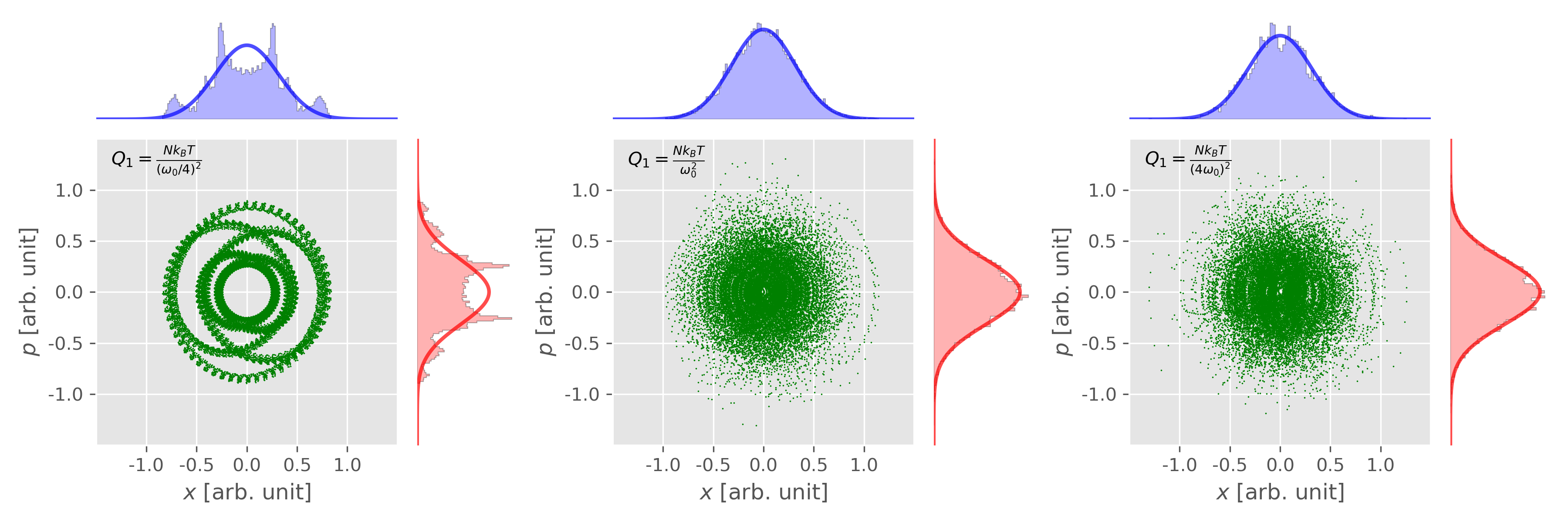
\[\begin{align} Q_1 &= {Nk_BT \over \omega_0^2} & \\[6pt] Q_k &= {k_BT \over \omega_0^2} & \quad 1 < k \le M \end{align}\]

Code Implementation

Below is the code that implement the Nosé-Hoover chain method to simulate the NVT ensemble for 1D harmonic oscillator, where an explicit time-reversible integrator is used. ⁸¹⁰¹¹

CLICK TO SHOW THE CODE!

#!/usr/bin/env python
# -*- coding: utf-8 -*-

import numpy as np


def harmonic_pot(x, m=1, omega=1):
    '''
    The harmonic potential
    '''

    return 0.5 * m * omega**2 * x**2

def harmonic_for(x, m=1, omega=1):
    '''
    The force of harmonic potential
    '''

    return - m * omega**2 * x

def Ekin(v, m=1):
    '''
    The force of harmonic potential
    '''

    return 0.5 * m * v**2

def log(x, v, m=1, omega=1):
    '''
    '''

    print("{:20.8E} {:20.8E} {:20.8E} {:20.8E} {:20.8E}".format(
        x, v,
        Ekin(v, m), 
        harmonic_pot(x, m, omega),
        harmonic_pot(x, m, omega) + Ekin(v, m)
    ))


def nose_hoover_chain(x0, v0, T, Q1, M=2, nc=1, nys=3, f0=None, m=1, omega=1, dt=0.01, nsteps=1000):
    '''
    G. J. Martyna, M. E. Tuckerman, D. J. Tobias, and Michael L. Klein,
    "Explicit reversible integrators for extended systems dynamics"
    Molecular Physics, 87, 1117-1157 (1996) 
    '''

    assert M >= 1
    assert nc >= 1
    assert nys == 3 or nys == 5

    if nys == 3:
        tmp = 1 / (2 - 2**(1./3))
        wdti = np.array([tmp, 1 - 2*tmp, tmp]) * dt / nc
    else:
        tmp = 1 / (4 - 4**(1./3))
        wdti = np.array([tmp, tmp, 1 - 4*tmp, tmp, tmp]) * dt / nc

    Qmass = np.ones(M) * Q1
    # if M > 1: Qmass[1:] /= 2
    Vlogs = np.zeros(M)
    Xlogs = np.zeros(M)
    Glogs = np.zeros(M)
    # for ii in range(1, M):
    #     Glogs[ii] = (Qmass[ii-1] * Vlogs[ii-1]**2 - T) / Qmass[ii]

    if f0 is None:
        f0 = harmonic_for(x0, m, omega)

    log(x0, v0, m, omega)


    def nhc_step(v, Glogs, Vlogs, Xlogs):
        '''
        '''

        scale = 1.0
        M     = Glogs.size
        K     = Ekin(v, m)
        K2    = 2*K
        Glogs[0] = (K2 - T) / Qmass[0]

        for inc in range(nc):
            for iys in range(nys):
                wdt = wdti[iys]
                # update the thermostat velocities
                Vlogs[-1] += 0.25 * Glogs[-1] * wdt

                for kk in range(M-1):
                    AA = np.exp(-0.125 * wdt * Vlogs[M-1-kk])
                    Vlogs[M-2-kk] = Vlogs[M-2-kk] * AA * AA \
                                  + 0.25 * wdt * Glogs[M-2-kk] * AA

                # update the particle velocities
                AA = np.exp(-0.5 * wdt * Vlogs[0])
                scale *= AA
                # update the forces
                Glogs[0] = (scale * scale * K2 - T) / Qmass[0]
                # update the thermostat positions
                Xlogs += 0.5 * Vlogs * wdt
                # update the thermostat velocities
                for kk in range(M-1):
                    AA = np.exp(-0.125 * wdt * Vlogs[kk+1])
                    Vlogs[kk] = Vlogs[kk] * AA * AA \
                              + 0.25 * wdt * Glogs[kk] * AA
                    Glogs[kk+1] = (Qmass[kk] * Vlogs[kk]**2 - T) / Qmass[kk+1]
                Vlogs[-1] += 0.25 * Glogs[-1] * wdt

        return v * scale

    # 0, 1, 2 represents t, t + 0.5*dt, and t + dt, respectively
    for ii in range(nsteps):
        vnhc = nhc_step(v0, Glogs, Vlogs, Xlogs)
        v1   = vnhc + 0.5 * dt * f0 / m
        x2   = x0 + v1 * dt
        f2   = harmonic_for(x2, m, omega)
        v2p  = v1 + 0.5 * dt * f2 / m
        v2   = nhc_step(v2p, Glogs, Vlogs, Xlogs)

        log(x2, v2, m, omega)
        x0, v0, f0 = x2, v2, f2

if __name__ == "__main__":
    T0 = 0.1
    v0 = np.sqrt(2*T0) * 2
    x0 = 0.0
    dt = 0.1
    N  = 20000

    nose_hoover_chain(x0, v0, T=T0, Q1=0.1, M=2, dt=0.1, nsteps=N)

Different chain lengths $M$

T0 = 0.1
v0 = np.sqrt(2 * T0) * 2
x0 = 0.0
dt = 0.1
N  = 20000
  
nose_hoover_chain(x0, v0, T=T0, Q1=0.1, M=1, dt=0.1, nsteps=N)
nose_hoover_chain(x0, v0, T=T0, Q1=0.1, M=2, nc=1, dt=0.1, nsteps=N)

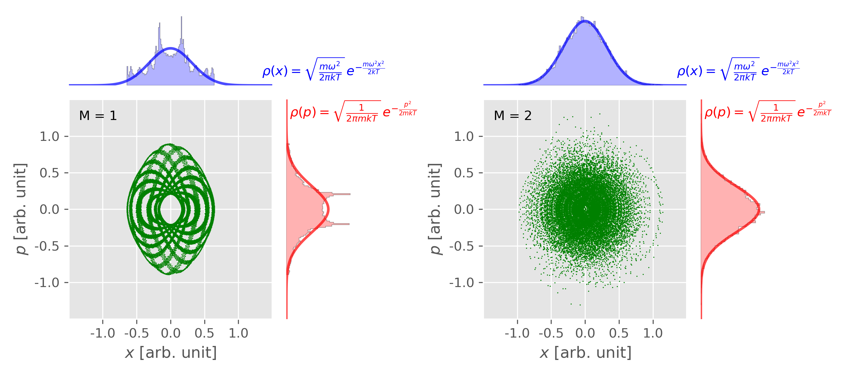
**Figure 4.** Phase space distribution of 1D harmonic oscillator obtained from NVT MD simulation with the Nosé-Hoover chain method. Left: NHC method with chain length $M = 1$; Right: NHC method with chain length $M = 2$. An explicit time-reversible integrator was used. Figure plotted using this script with this input data.

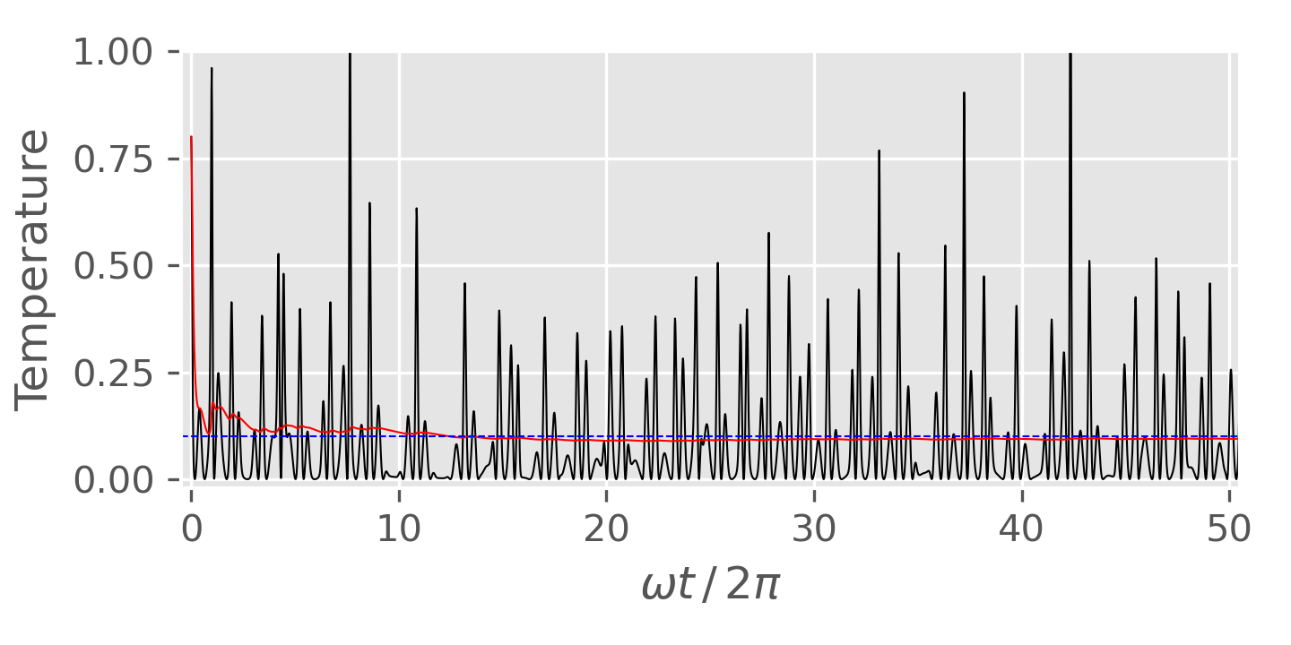
**Figure 5.** Temperature fluctuation of 1D harmonic oscillator obtained from NVT MD simulation with the Nosé-Hoover chain method (chain length: $M=2$). The black solid line is the instantaneous temperature and the red line is the averaged temperature. The blue horizontal line shows the target temperature. Figure plotted using this script with this input data.

Different initial condictions for $M = 1$
1 2 3 4 5 6 T0 = 0.1 dt = 0.1 N = 20000 for x0, v0 in np.mgrid[0:3, 0:3].reshape((2, -1)).T * np.sqrt(2*T0): nose_hoover_chain(x0, v0, T=T0, Q1=0.1, M=1, dt=0.1, nsteps=N)
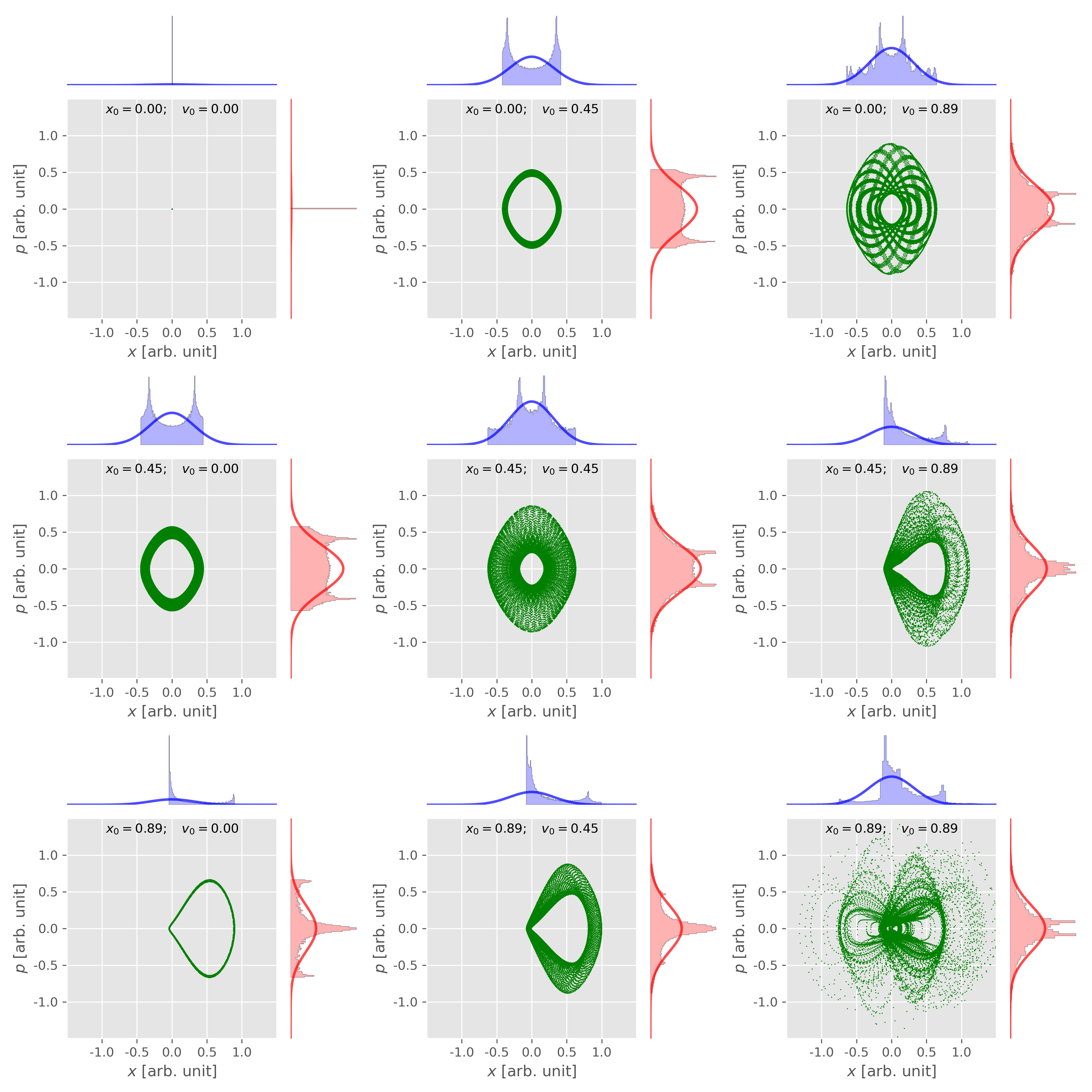
Figure 6. The phase space distribution of 1D harmonic oscillator from Nose-Hoover thermostat ($M = 1$) depends on the initial conditions. Figure plotted using this script with this input data.

Different thermal inertia $Q_1$

T0 = 0.1
x0 = 0.0
v0 = np.sqrt(2 * T0) * 2
dt = 0.1
N  = 20000

nose_hoover_chain(x0, v0, T=T0, Q1=0.1 * 16, M=2, nc=1, dt=0.1, nsteps=N)
nose_hoover_chain(x0, v0, T=T0, Q1=0.1, M=2, nc=1, dt=0.1, nsteps=N)
nose_hoover_chain(x0, v0, T=T0, Q1=0.1 / 16, M=2, nc=1, dt=0.1, nsteps=N)

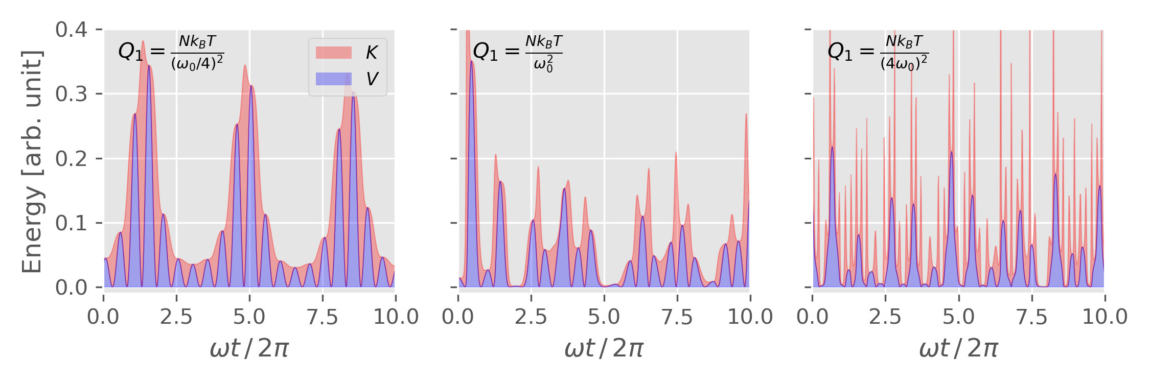
**Figure 8.** Potential energy and kinetic energy of 1D harmonic oscillator from Nose-Hoover chain thermostat ($M = 2$) with different "thermal inertia" $Q_1$. Figure plotted using this script with this input data.

References

Daan Frenkel and Berend Smit, Understanding Molecular Simulation: From Algorithms to Applications ↩ ↩² ↩³ ↩⁴
Cameron Abrams, Drexel University, Molecular Simulations ↩
Shuichi Nosé, J. Chem. Phys., 81, 511(1984). ↩ ↩² ↩³ ↩⁴
William G. Hoover, Phys. Rev. A, 31, 1695(1985). ↩ ↩²
Mark E. Tuckerman, Statistical Mechanics: Theory and Molecular Simulation ↩
Mark E. Tuckerman and Glenn J. Martyna, Understanding Modern Molecular Dynamics: Techniques and Applications, J. Phys. Chem. B, 104, 159–178(2000) ↩
Glenn J. Martyna and Michael L. Klein, Nosé–Hoover chains: The canonical ensemble via continuous dynamics, J. Chem. Phys., 97, 2635(1992) ↩
G. J. Martyna, M. E. Tuckerman, D. J. Tobias, and Michael L. Klein, Explicit reversible integrators for extended systems dynamics, Molecular Physics, 87, 1117-1157 (1996) ↩ ↩² ↩³
I am not sure why this Q is different from that in Eq.\eqref{eq:suggestedQ}. ↩
https://github.com/google/jax-md ↩
openmmtools.integrators.NoseHooverChainVelocityVerletIntegrator ↩

Molecular Dynamics at Constant Temperature

Canonical Ensemble

Velocity Rescaling

Stochastic Thermostat

Andersen Thermostat

Langevin Thermostat

Velocity-Verlet algorithm for Langevin thermostats

Extended Lagrangian Method

Nosé-Hoover Thermostat

EOM in virtual variables

EOM in real variables

Pros & Cons

Nosé-Hoover Chains

Code Implementation

References

Further Reading

PAW All-Electron Wavefunction in VASP

Light-Matter Interaction and Dipole Transition Matrix

Band Unfolding Tutorial

Trending Tags